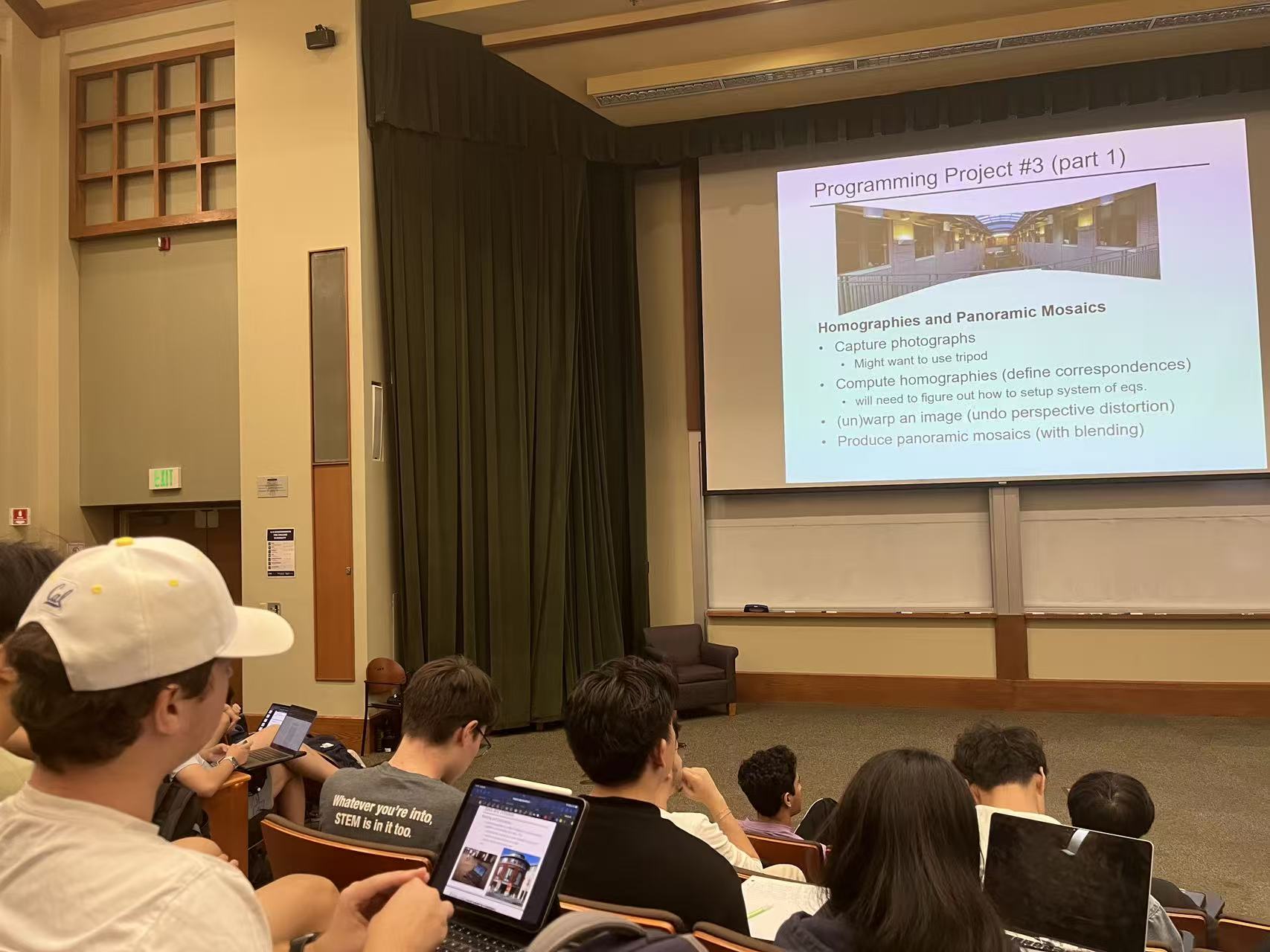
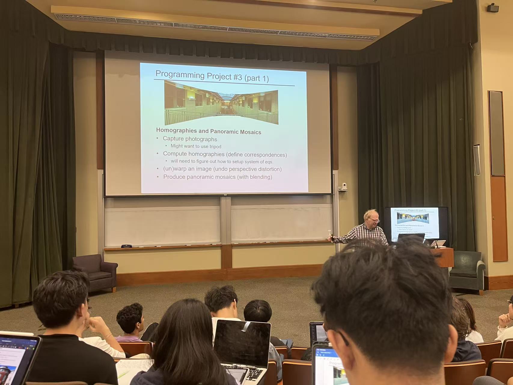
Project 3: [Auto]Stitching Photo Mosaics
Project Overview
This project implements the automatic stitching of photo mosaics. For part A, the stitching is done by manually picking correspondence points between the images and using a homography matrix to project the images on the same plane.
Part A.1: Shoot the Pictures
This part includes sets of pictures shot with projective transformations, ie. rotating the camera while keeping the COP (center of projection) the same. Later part of the project will be done with these pictures.
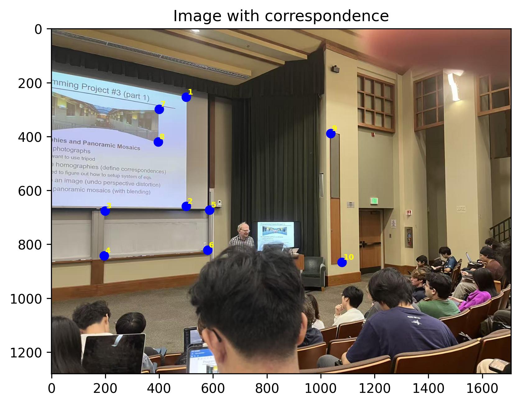
During Lecture (left)
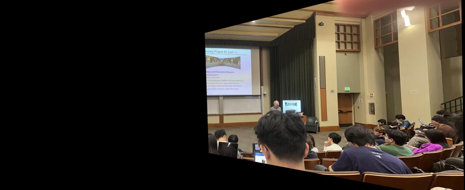
During Lecture (middle)
During Lecture (right)

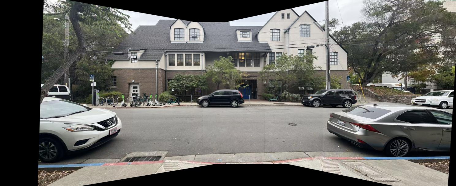
Outside Soda (left)
Outside Soda (middle)
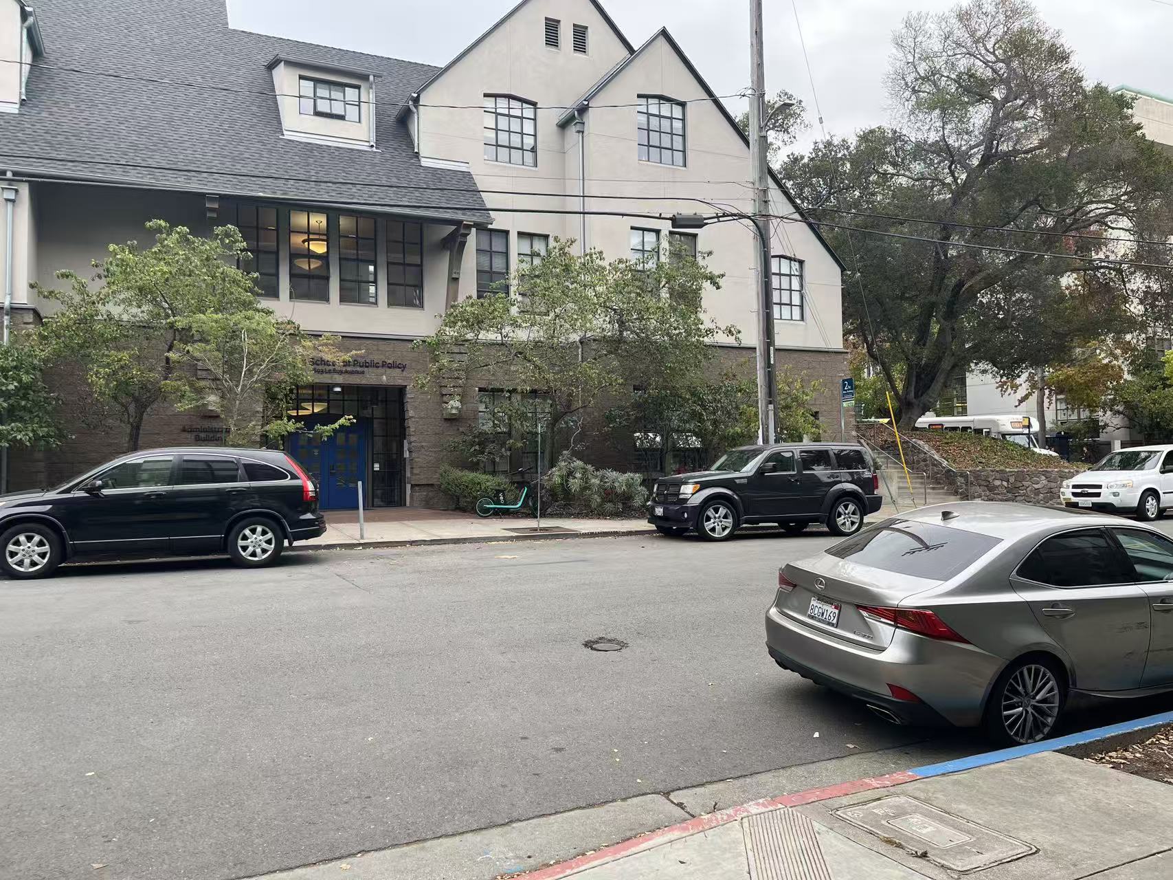
Outside Soda (right)
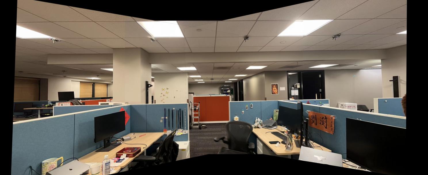
Inside Sky Lab (left)
Inside Sky Lab (middle)
Inside Sky Lab (right)
Part A.2: Recover Homographies
This part introduces how we can recover the homography matrix with a set of correspondence points. Note that the homography matrix has 8 degrees of freedom, therefore we need at least 4 points to recover a homography matrix. More points are needed for a more robust recovery.
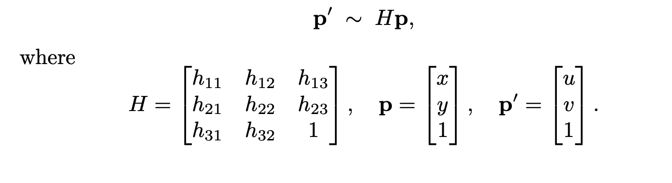
Homography Matrix
Since the 1 on the homography matrix is fixed, we cannot directly solve for the homography matrix. Therefore, we need to expand the system of equations and use least squares to solve for the homography matrix.
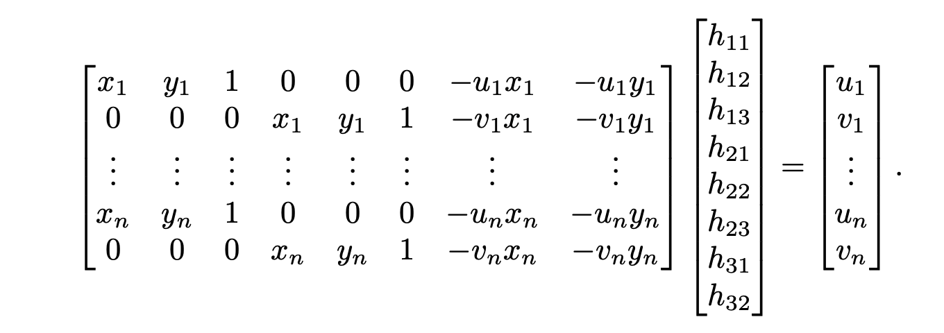
System of Equations to Recover the Homography matrix
An example of manually picked correspondences and the recoevred homography matrix are shown below.
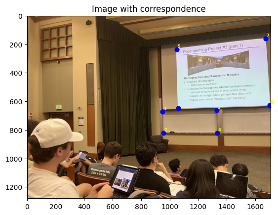
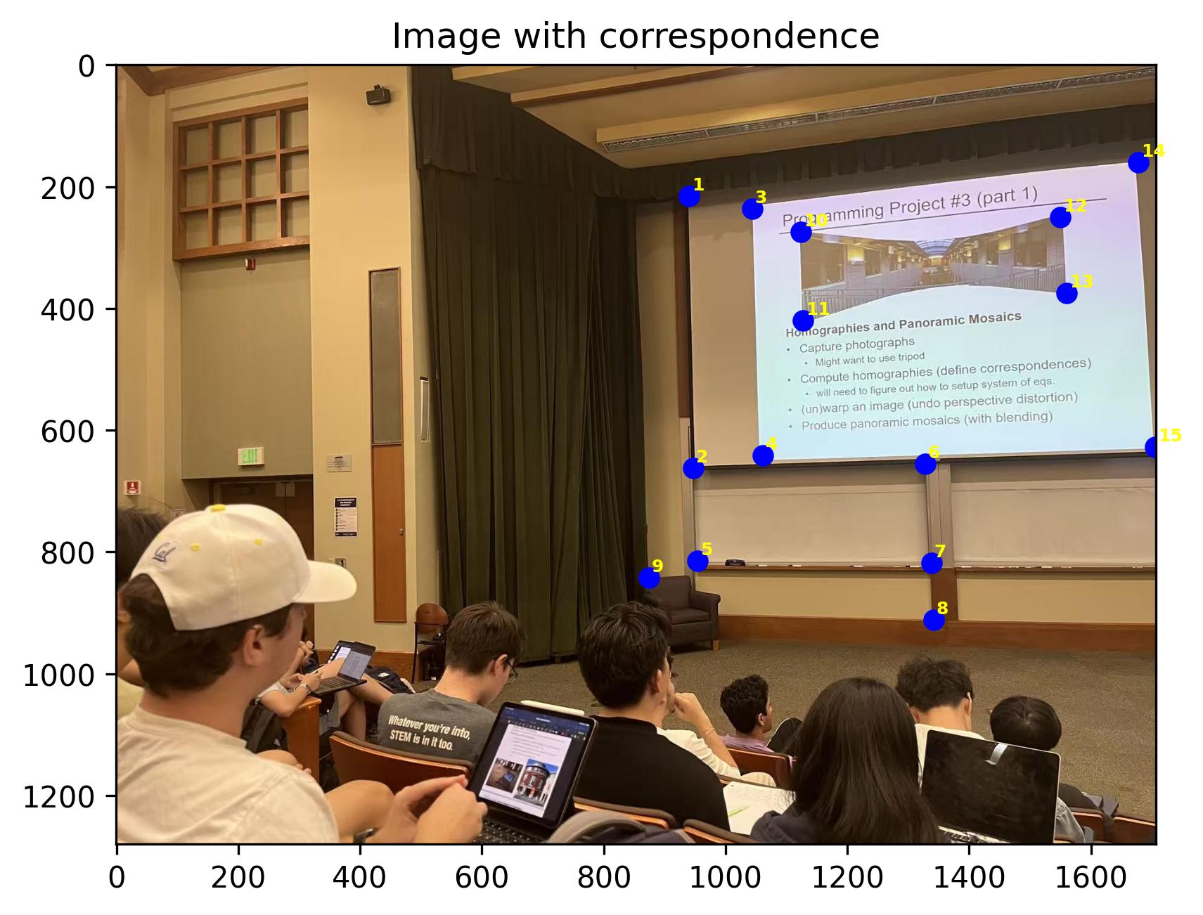
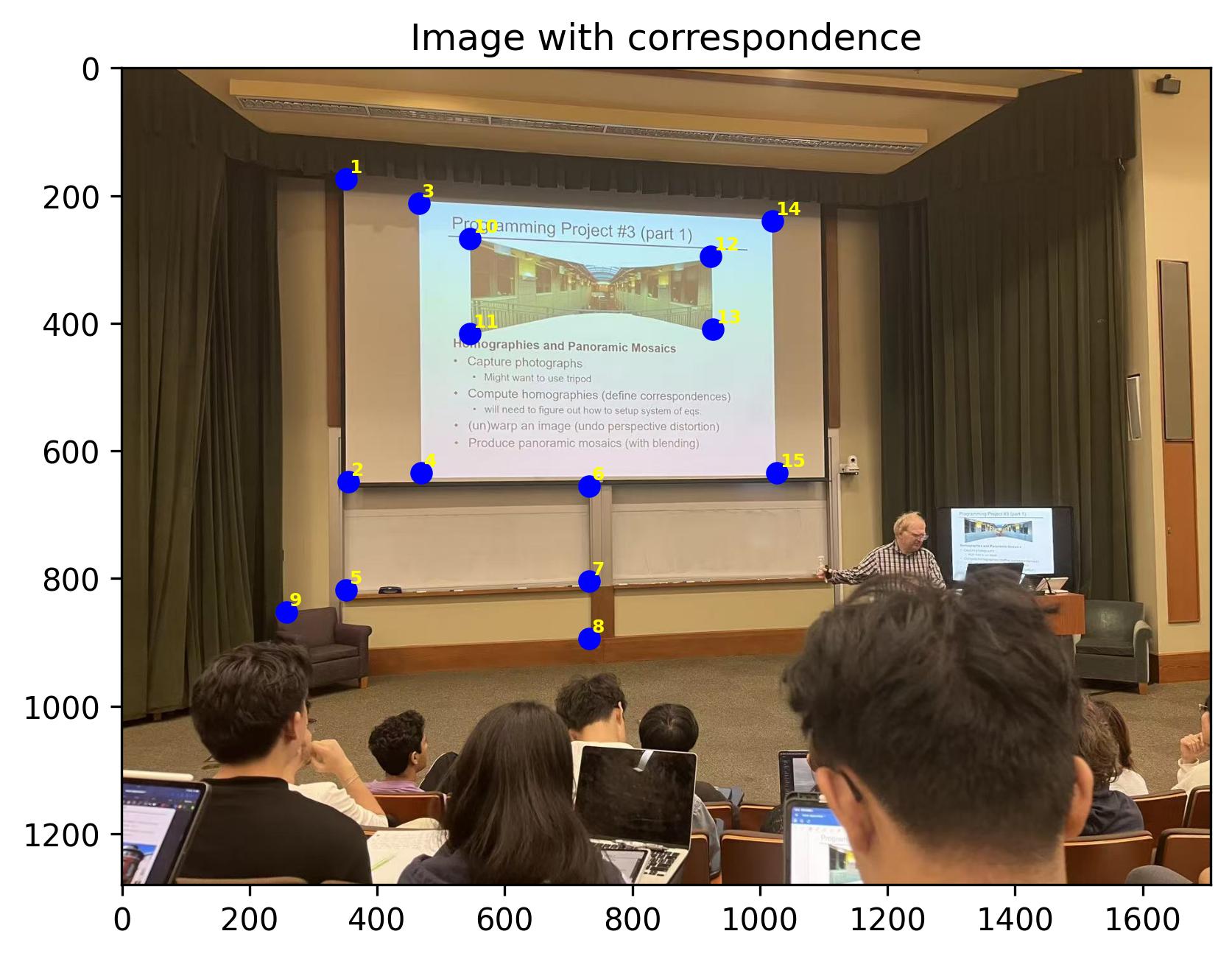
During Lecture (left) Correspondences

During Lecture (middle) Correspondences
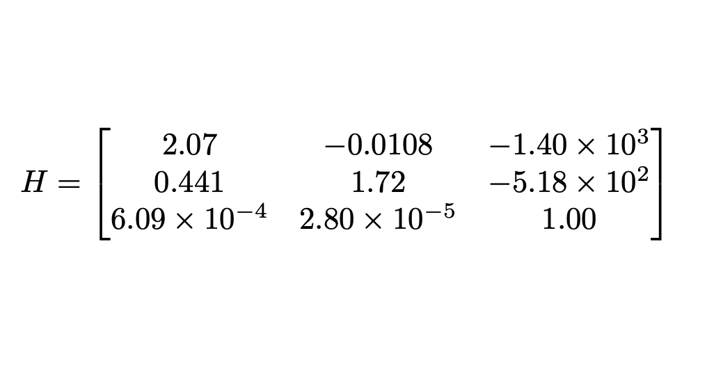
The Recovered Homography Matrix
Part A.3: Warp the Images
This part introduces two methods to warp the images after recovering the homography matrix: nearest neighbor and bilinear interpolation. The nearest neighbor method is the simplest method to warp the images, where one only needs to find the pixel values of the nearest pixel in the original image (pixels are got from inverse mapping); he bilinear interpolation method finds the pixel values of the four nearest pixels in the original image and uses a weighted average to find the pixel values of the warped image. Here are some examples of the warped images (rectification) with both methods.
Channing Court at 7 AM
Warped Channing Court (Nearest Neighbor)
Warped Channing Court (Bilinear Interpolation)
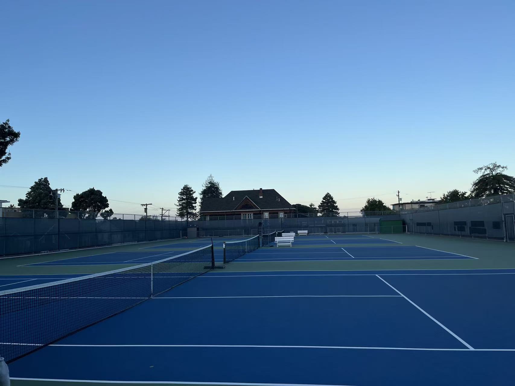
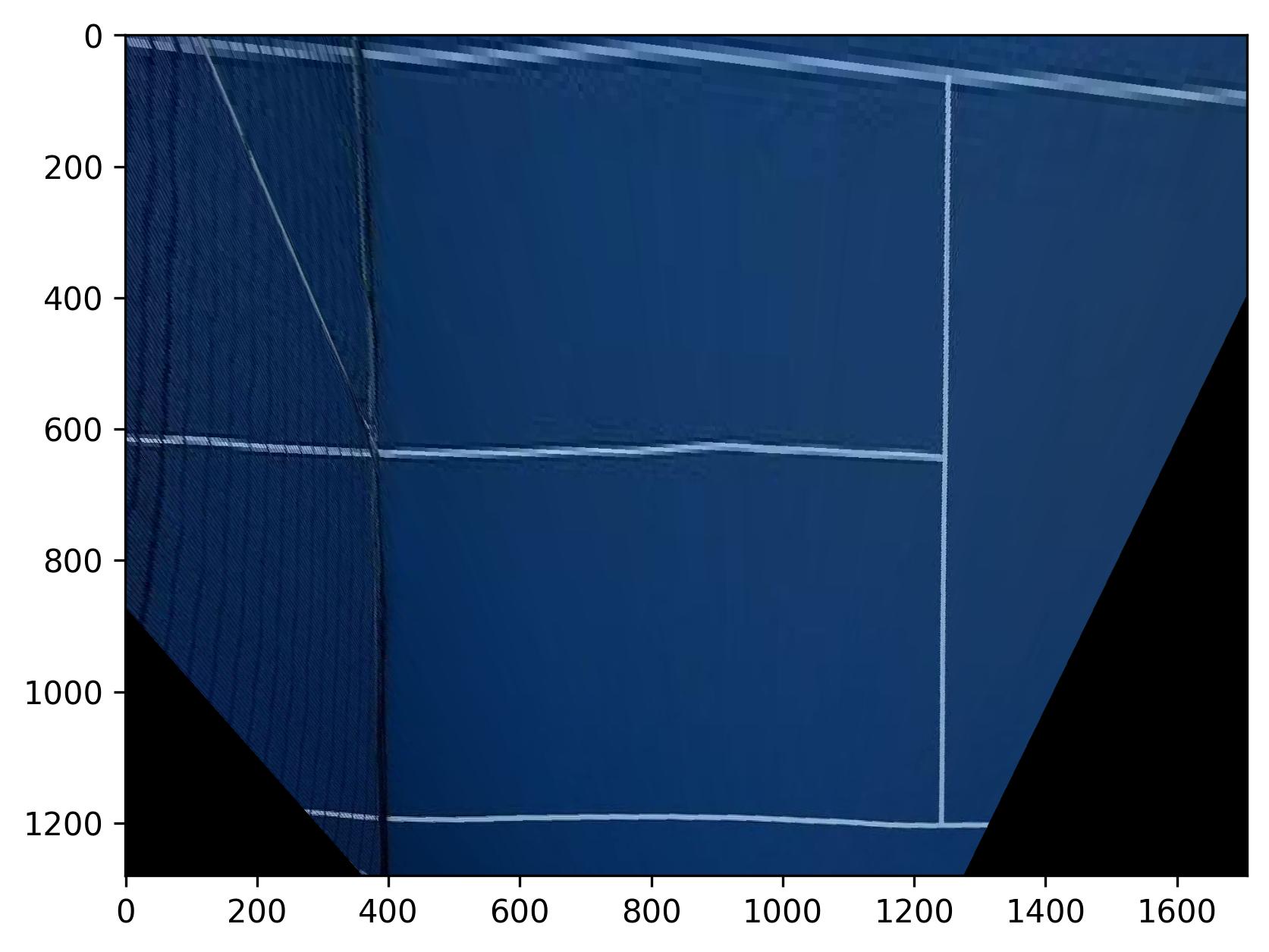
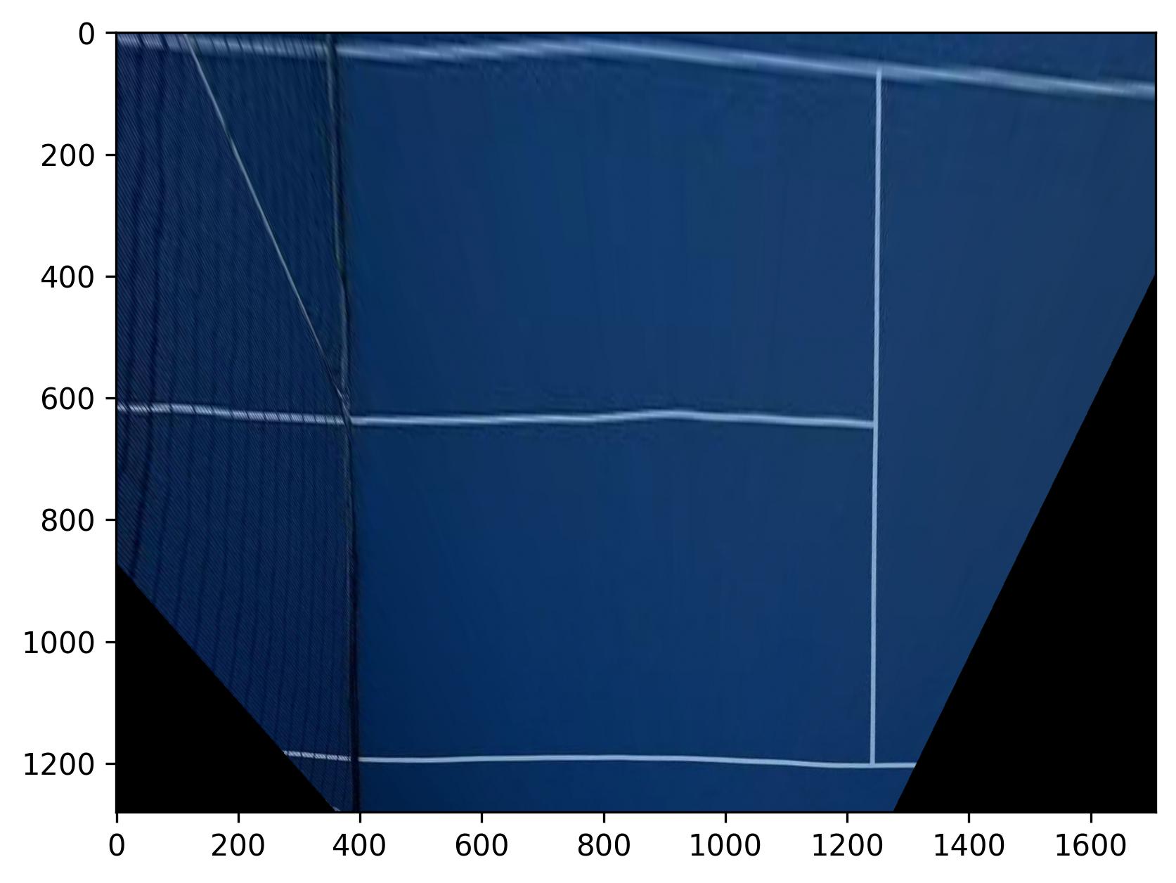
Roomates

Warped Roomates (Nearest Neighbor)
Warped Roomates (Bilinear Interpolation)
What? Lines in a tennis court are not straight? That is probably because of the distortion with the camera in the original image.
Note that the nearest neighbor warping results in more artifacts than the bilinear interpolation method, an example can be found at the top of the warped channing court image.
Part A.4:Blend the Images into a Mosaic
This part of the project blends the images into a mosaic. The procedure is simple:
- Manually pick correspondences between the images
- Pad the images with thick black borders so that we can have better view of the whole stitched image
- Use the picked points to recover a homography matrix
- Warp the images to the same plane
- Add a mask used for blending
- Blend the images into a mosaic using a weighted average calculated with the mask. To be more specific, I take the average of the images where the masks overlap with each other.
Below are some examples of the stitched images. The first set of images will be used as an example to demonstrate the procedure, and the intermediate results for the other two sets of images will not be shown here for brevity.
During Lecture (left) Correspondences
During Lecture (middle) Correspondences
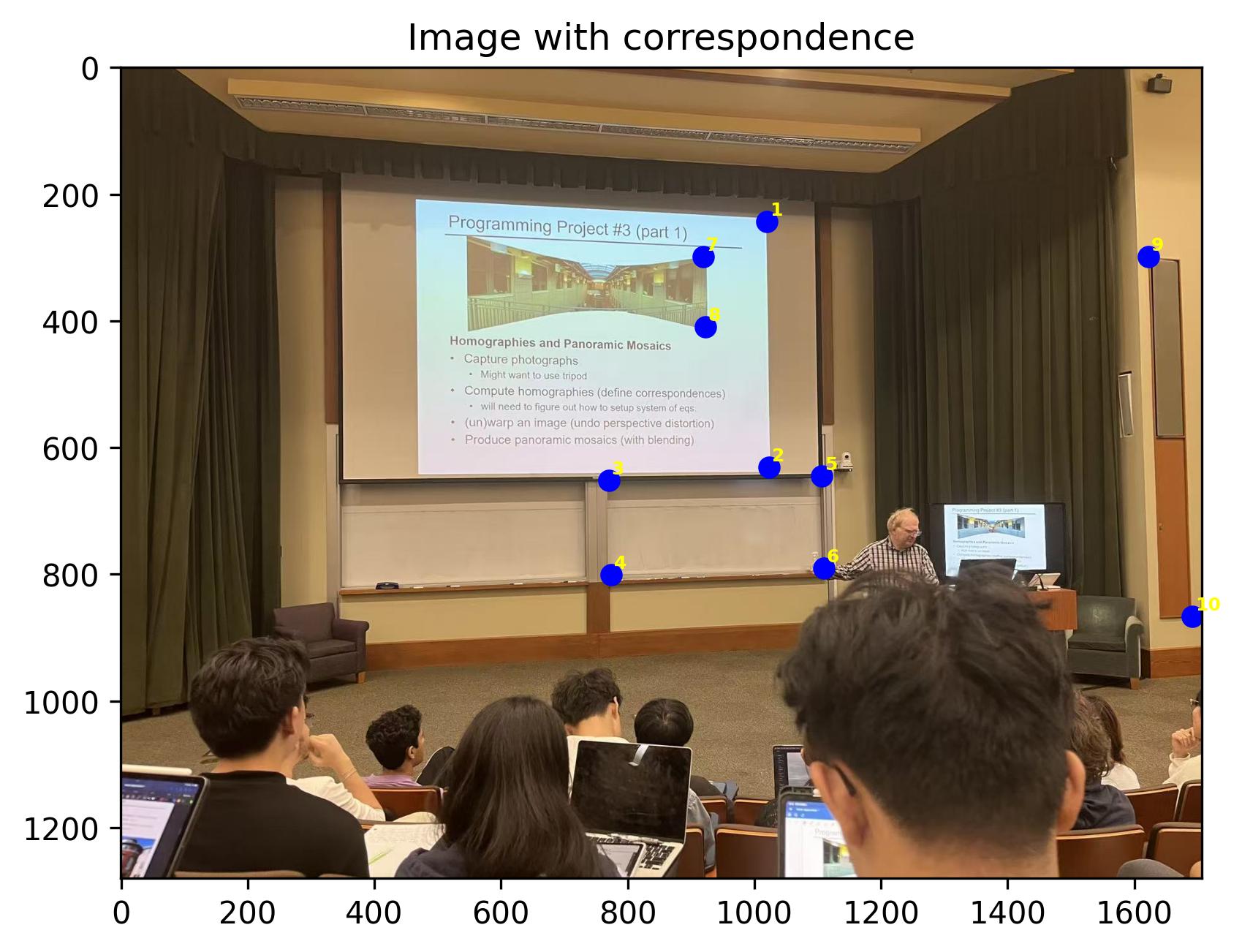
During Lecture (middle for right) Correspondences
During Lecture (right) Correspondences
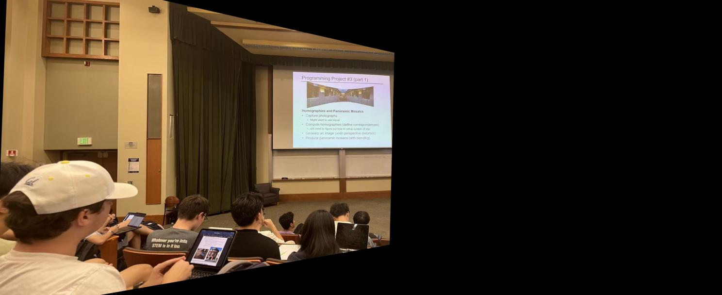
Warped Lecture (left)
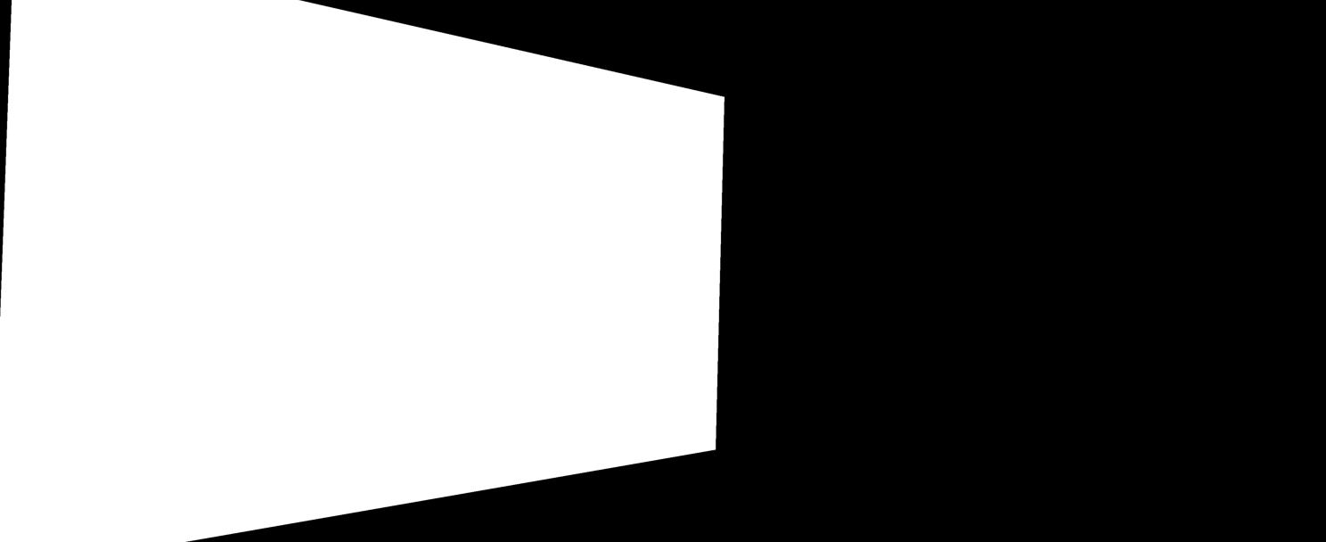
Mask for Lecture (left)
Warped Lecture (middle)
Mask for Lecture (middle)
Warped Lecture (right)
Mask for Lecture (right)
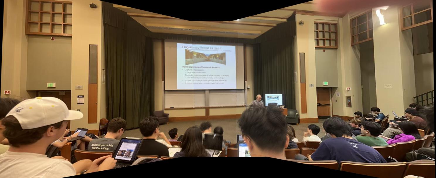
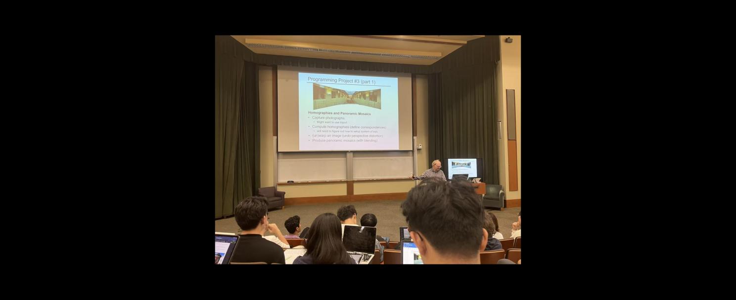
During Lecture
Outside Soda (left)
Outside Soda (middle)
Outside Soda (right)
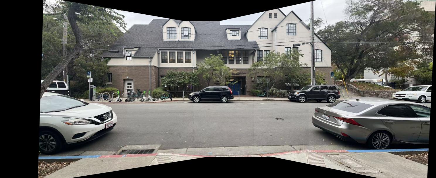
Outside Soda
Inside Sky Lab (left)
Inside Sky Lab (middle)
Inside Sky Lab (right)
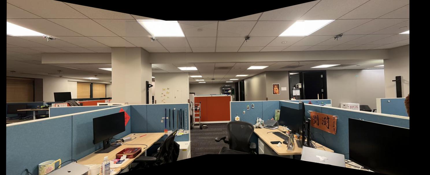
Inside Sky Lab
Part B.1: Harris Corner Detection
In this section, I use the Harris corner detection algorithm to detect the corners of the images. However, naively choosing the strongest corners will lead to a uneven distribution of the features. Therefore, I applied Adaptive Non-Maximal Suppression (ANMS) to choose the corners. The following images are the results of the Harris corner detection and the Adaptive Non-Maximal Suppression.
ANMS is implemented by the following steps:
- Detect the corners of the image using the Harris corner detection algorithm and sort the corners by the Harris response score
- Maintain a list of already selected corners, initialized as empty
- for the i-th corner, calculate the minimum distance to the already selected corners with a response score threshold of 0.9
- Sort the corners by the minimum distance and select the top k corners
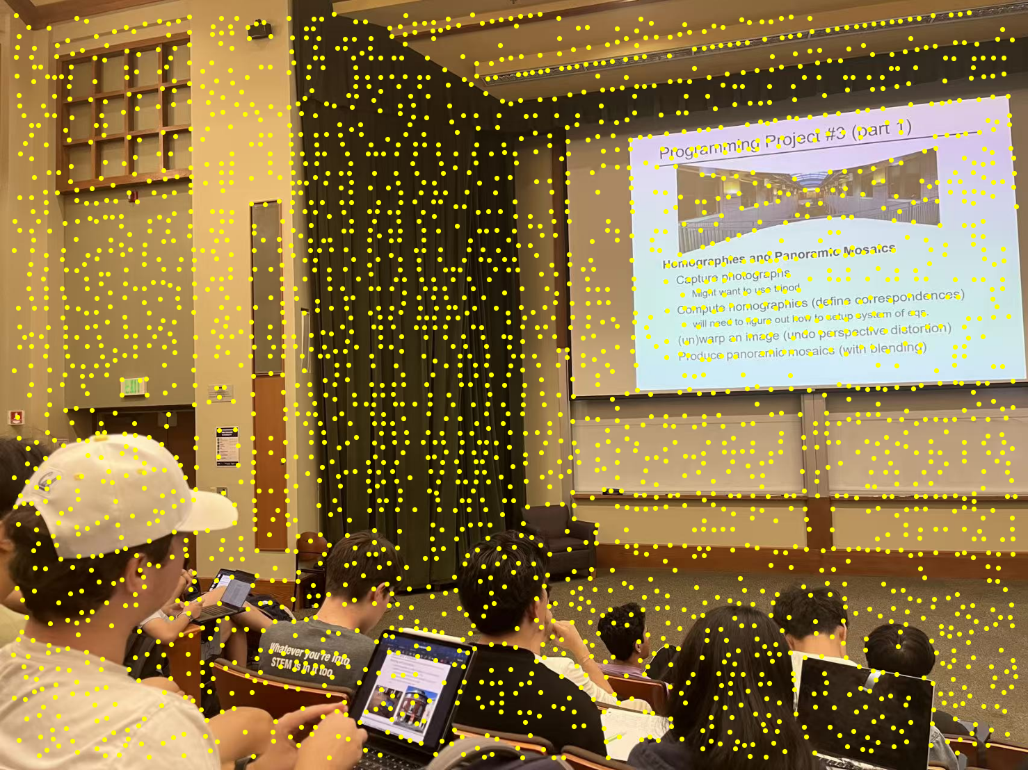
Lecture 1 with all corners detected by Harris corner detection

Lecture 1 with 500 strongest corners

Lecture 1 with 500 corners selected by ANMS
Part B.2: Feature Descriptor Extraction
This part of the project implements the feature descriptor extraction. The feature descriptor is a 8 by 8 square patch, downsampled from a 40 by 40 patch on the original scale. All the descriptors here are axis-aligned since no rotation is involved in taking the pictures. The following images are some examples of the feature descriptors from the left lecture image.
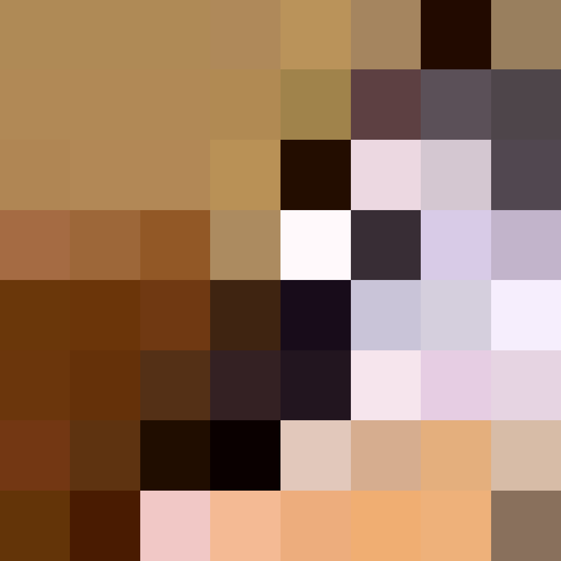
Lecture Descriptor Patch Example 1
Lecture Descriptor Patch Example 2
Lecture Descriptor Patch Example 3
Part B.3: Feature Matching
This part of the project implements the feature matching process. The feature matching is done by iterating through all the feature descriptors; for each descriptor, track the ratio between the errors of the best and the second best match. If the ratio is less than 0.7, then we consider it as a good match.
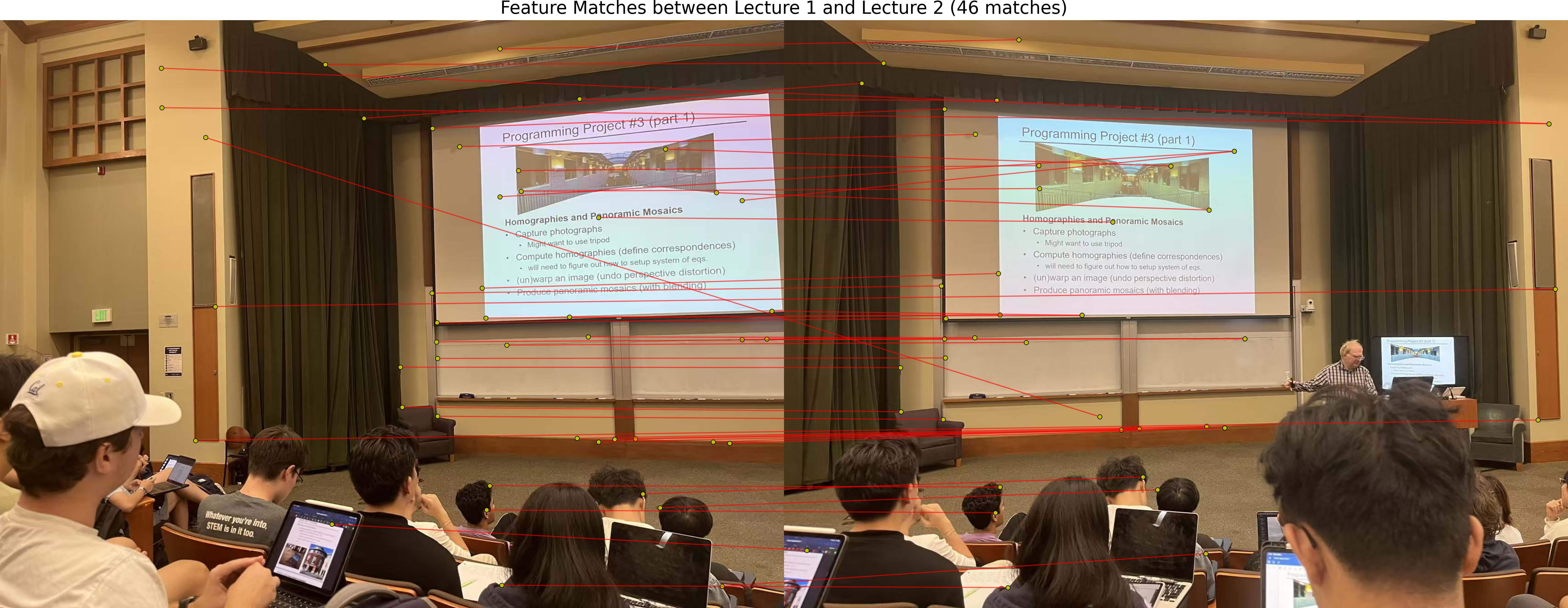
Lecture Matches
Part B.4: RANSAC for Robust Homography
This part of the project implements the RANSAC algorithm to robustly estimate the homography matrix. The RANSAC algorithm is implemented by the following steps:
- Randomly sample 4 points from the matches
- Estimate the homography matrix using the 4 points
- Count the number of inliers
- Repeat the process for a certain number of iterations
- With the most inliers, estimate the homography matrix with all the inliers
- Return the homography matrix
The following images are some examples of the auto-stitched images and a comparison between the stitching with manually picked correspondences.
During Lecture (Stitched Manually)
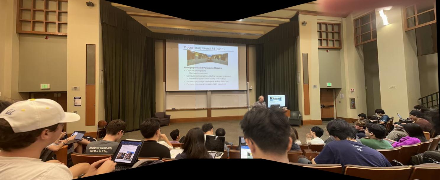
During Lecture (Stitched with RANSAC)
Outside Soda (Stitched Manually)
Outside Soda (Stitched with RANSAC)
Inside Sky Lab (Stitched Manually)
Inside Sky Lab (Stitched with RANSAC)