Part 0: Calibrating Your Camera and Capturing a 3D Scan
This part calibrates the cameta, captures the images for the object, and undistorts them for later reconstrcution.
The following images show the cloud of cameras visualized with Viser and the difference between the original images and the undistorted images.
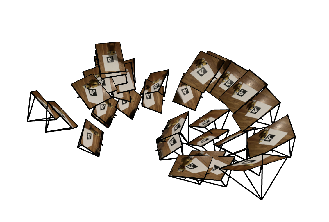
Image 1 for the captured Dataset
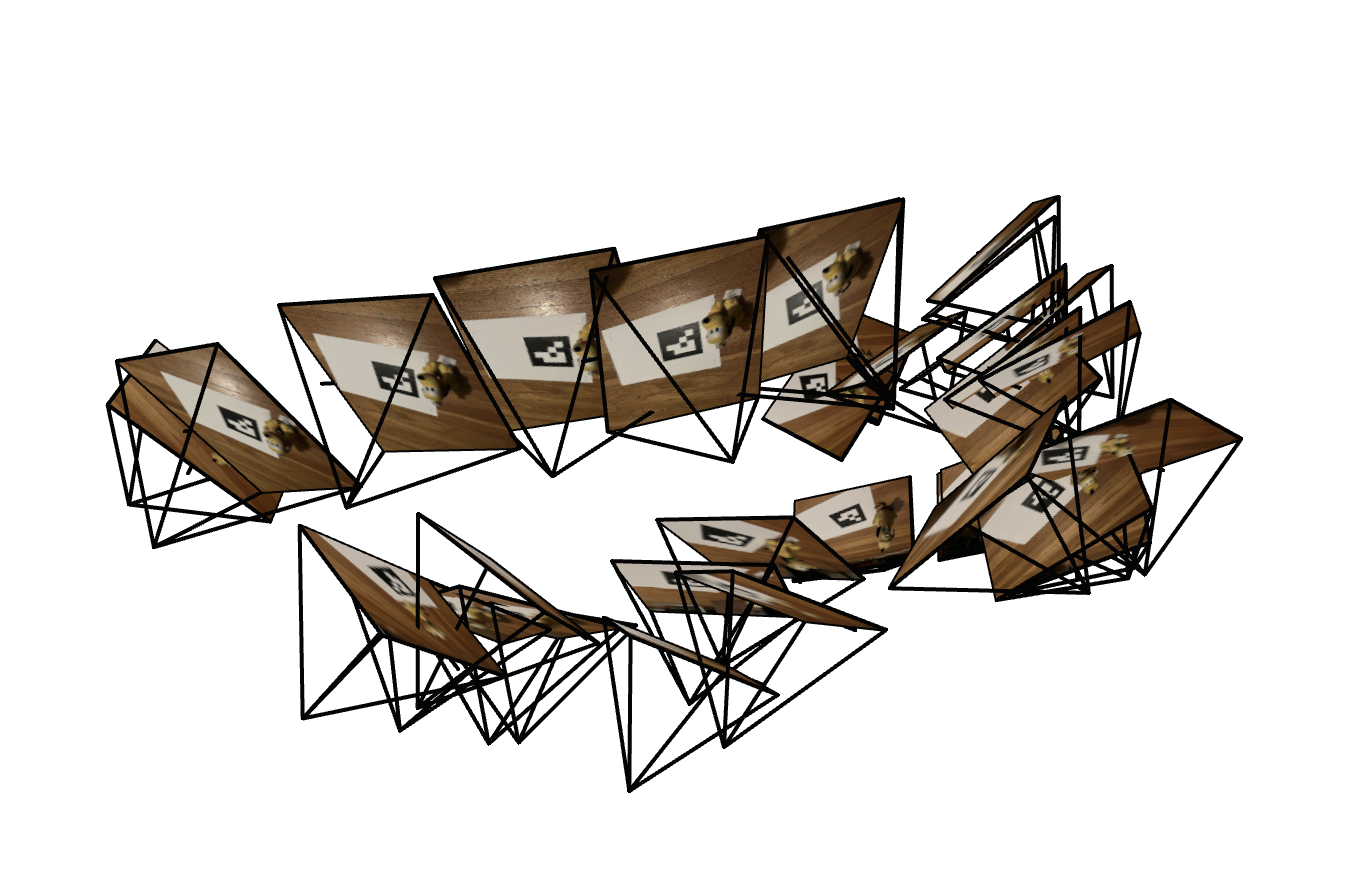
Image 2 for the captured Dataset
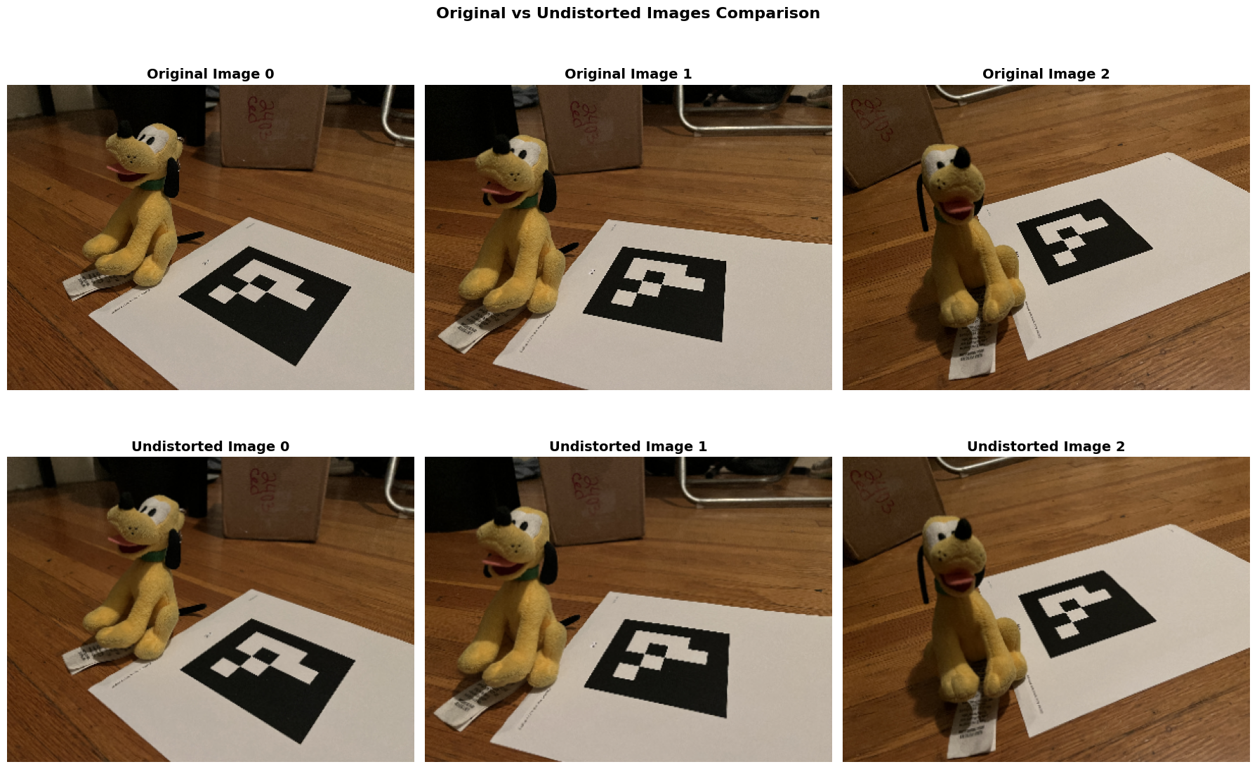
comparison between the original and the undistorted images
Part 1: Fit a Neural Field to a 2D Image
To get started, we first fit a neural field to a 2D image. The coordinates are first transformed into positional embeddings, and then passed in a MLP. The MLP is constructed with 4 linear layers interleaved with ReLU functions, with a sigmoid function after the final layer. Adam is used as the optimizer with a learning rate of 0.01.
The frequency of the positional embeddings and the size of the linear layer are varied to see how these two factors affect the reconstrcution quality.
Images are also reconstructed at the checkpoints and are shown below. The PSNR curve from training is also shown below. The final reconstructed image is shown in the final checkpoint column.
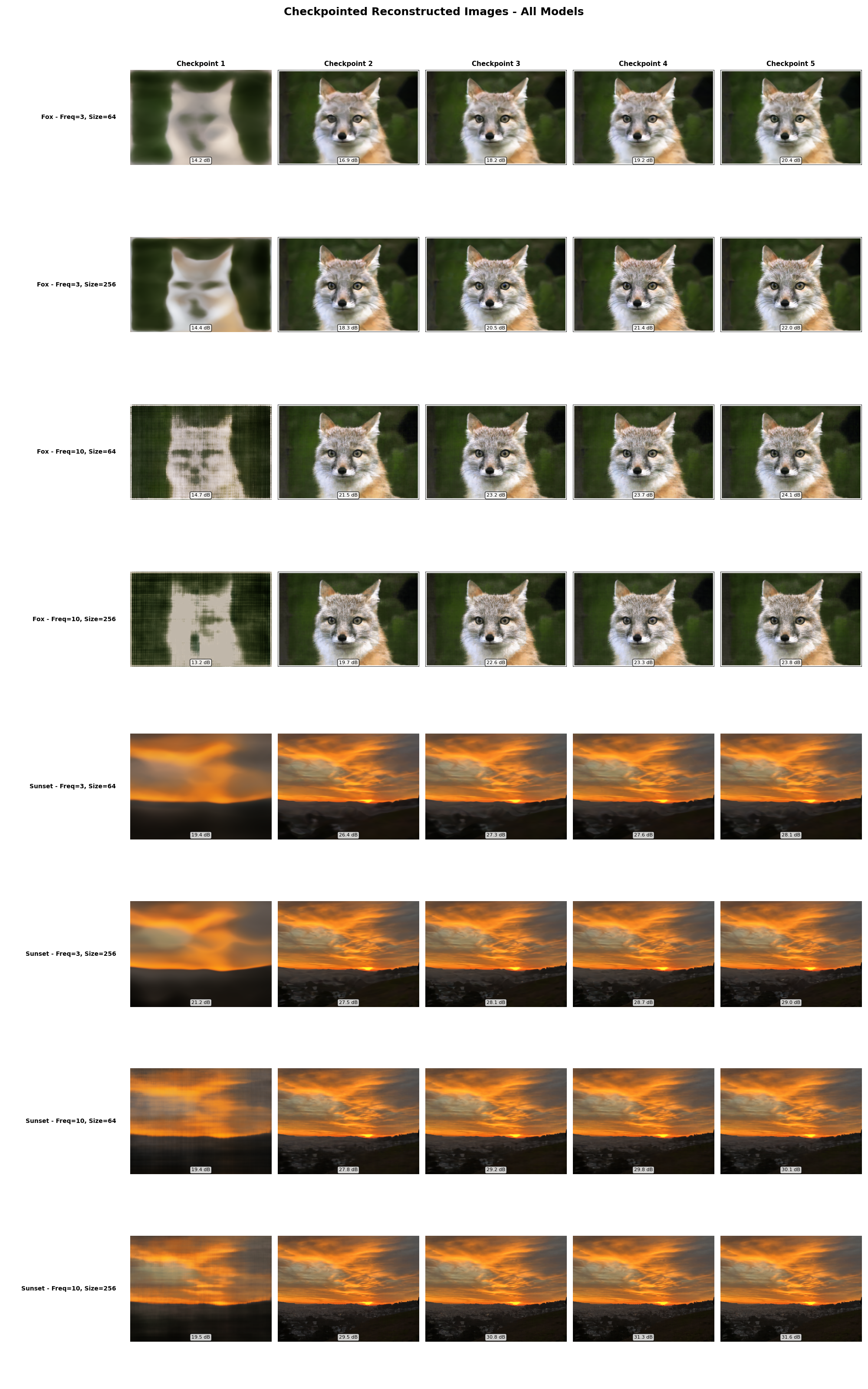
2D Image Reconstrcution
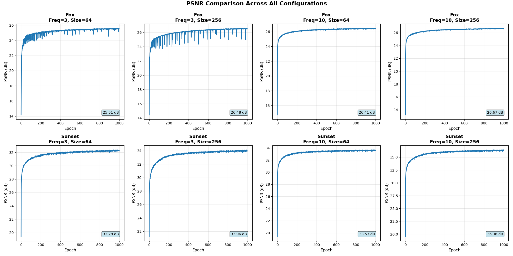
Training PSNR Curve
Part 2: Fit a Neural Radiance Field from Multi-view Images
We separately implement the following functions: transform, pixel_to_camera, pixel_to_ray for part 2.1. All functions are implemented in batched operation. The transform function implements a basic matrix vector multiplication, truncating the homogenous coordinates. The pixel_to_camera function converts pixel coordinates to camera coordinates (note that this correponds to a ray, which is why we need a scale argument to fix the point), and the pixel_to_ray function generates rays from the camera coordinates.
For part 2.2, we implement different sampling procedures. For the sample_ray_from_images function, we first sample pixels from the image and then use the pixel_to_ray function to generate the rays. We also sample points along the rays, where we uniformly select num_sample points between the arguments near and far, with optional random perturbation.
For part 2.3, we implement the RayDataset, and visualize the rays with Viser. Pictures of the rays sampled from the bulldozer images are shown below.
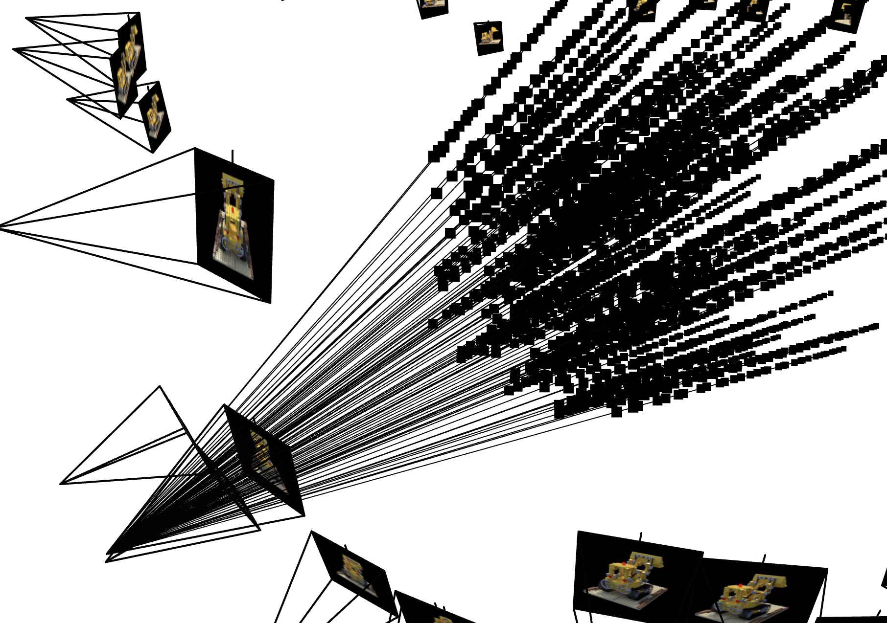
Ray Visualization from a Single Image
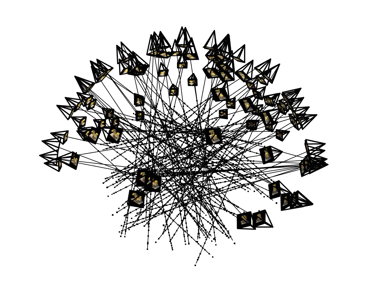
100 Rays sampled from all the Images
Finally, we implement the NeRF model with the following architecture in part 2.4.
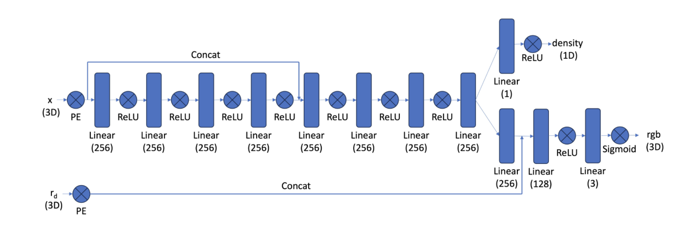
Model Architecture
In part 2.5, we implement the volume rendering function, taking in a list of predicted RGB values and densities and outputting the predicted reconstructed pixel. Using the cumprod function in PyTorch for calculating the T_i values speed up the computation.
The following images visualize the training process, the validation PSNR curve, and the final reconstructed 3D bulldozer.
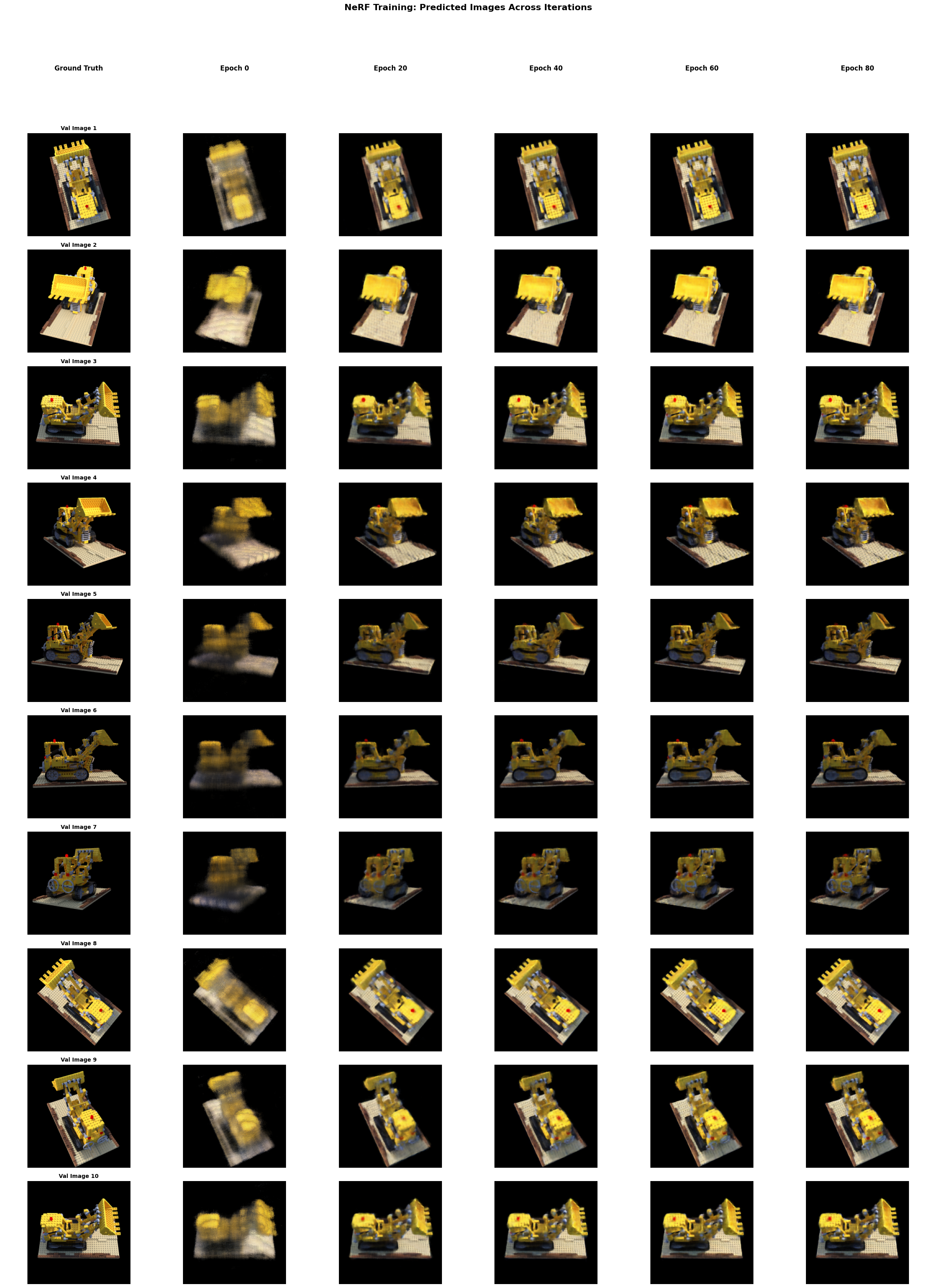
Training Progression
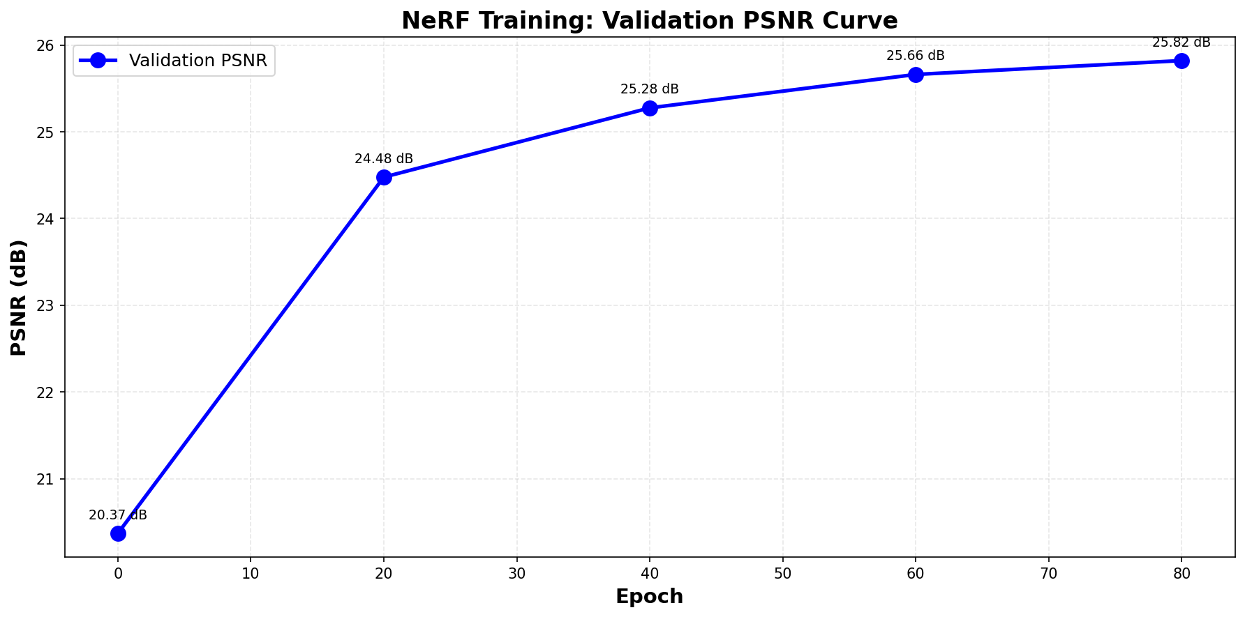
PSNR values evaluated on the validation set
Reconstrcution of the Bulldozer
Part 2.6: Training with My Own Data
This part of the project trains a NeRF model on my own data captured with my iPhone 13. The model architecture stays the same as the previous part. The only hyperparameters changed are the near and far values used when sampling the points along the ray.
Note that the quality of the reconstruction is low due to the fact that the tags are hidden behind the object in some directions, and therefore we lack the data from those directions.
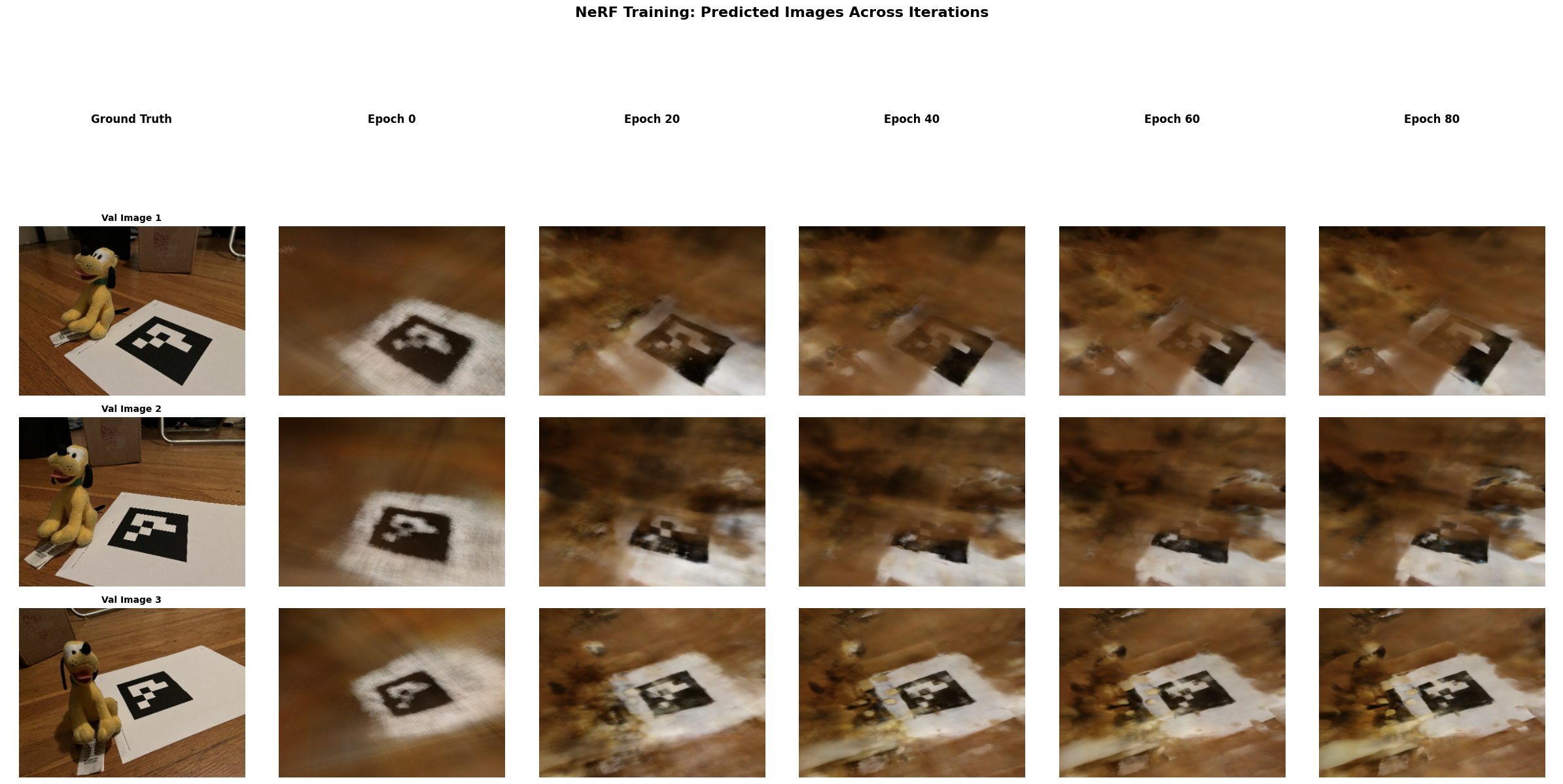
Training Progression for my NeRF Data
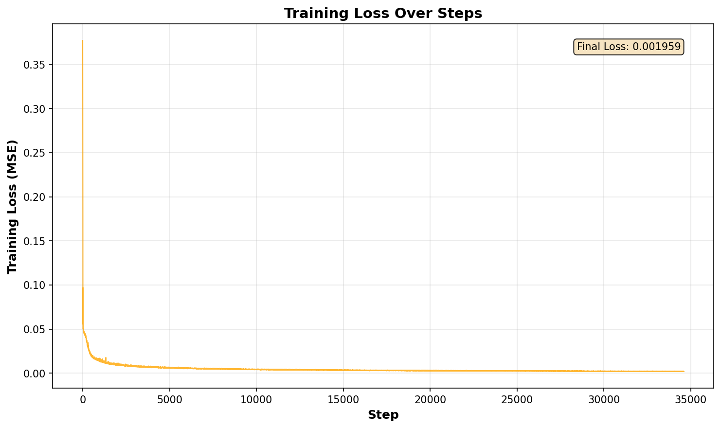
Training Loss
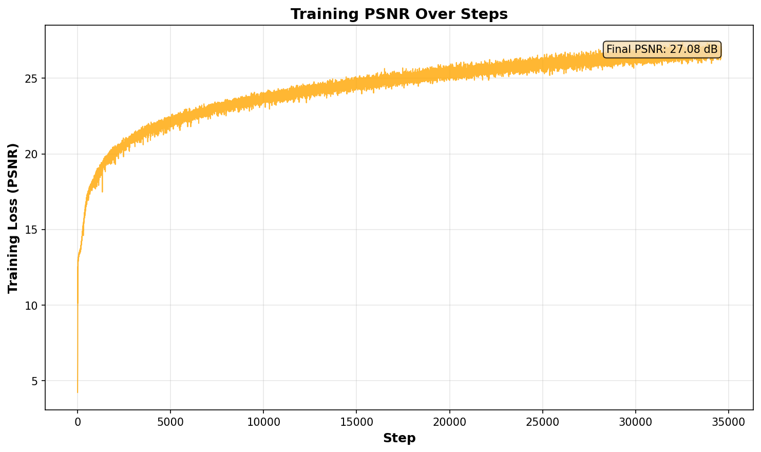
Training PSNR
Reconstrcution of my own Data
Note that due to the low quality of the reconstruction, I will include a reconstructed Lafufu with the staff captured dataset, proving the point that my implementation is flawless.
Reconstrcution of the Staff Data