Project 5: Fun with Diffusion Models

Part 0: Setup and Playing with my own Text Prompt

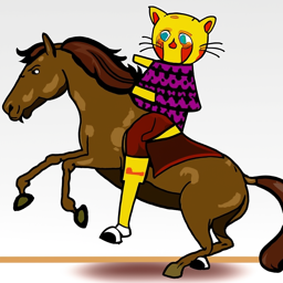
This part sets up the environment and plays with my own text prompt. We can observe that for prompts that are too abstract or OOD, the generated images are not very good. However, for prompts that are more specific and in-domain, the generated images are much better. The seed chosen is here is 100 for reproducibility.

The first row shows the generated image with a inference step of 50, while the second row shows the generated image with a inference step of 100.

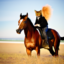
"a cat riding a horse", step 50

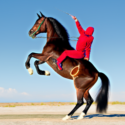
"a horse riding a cat", step 50

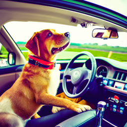
"a dog driving a car", step 50

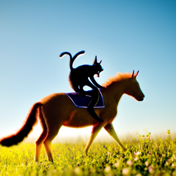
"a cat riding a horse", step 100

"a horse riding a cat", step 100

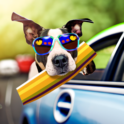
"a dog driving a car", step 100

Part 1.1 and Part 1.2: Forward Pass and Classical Denoising

Part 1.1 implements the forward pass by adding noise according to the noise schedule. The formula used for the forward pass is given by:

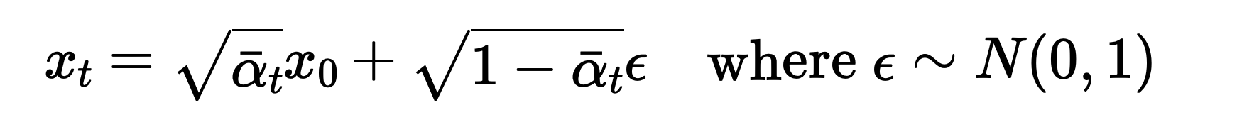
Forward Pass

Part 1.2 implements the classical denoising by simply passing the noisy images through a gaussian filter. The comparison and the results from part 1.1 are shown below. images are taken at time steps 250, 500, 750.

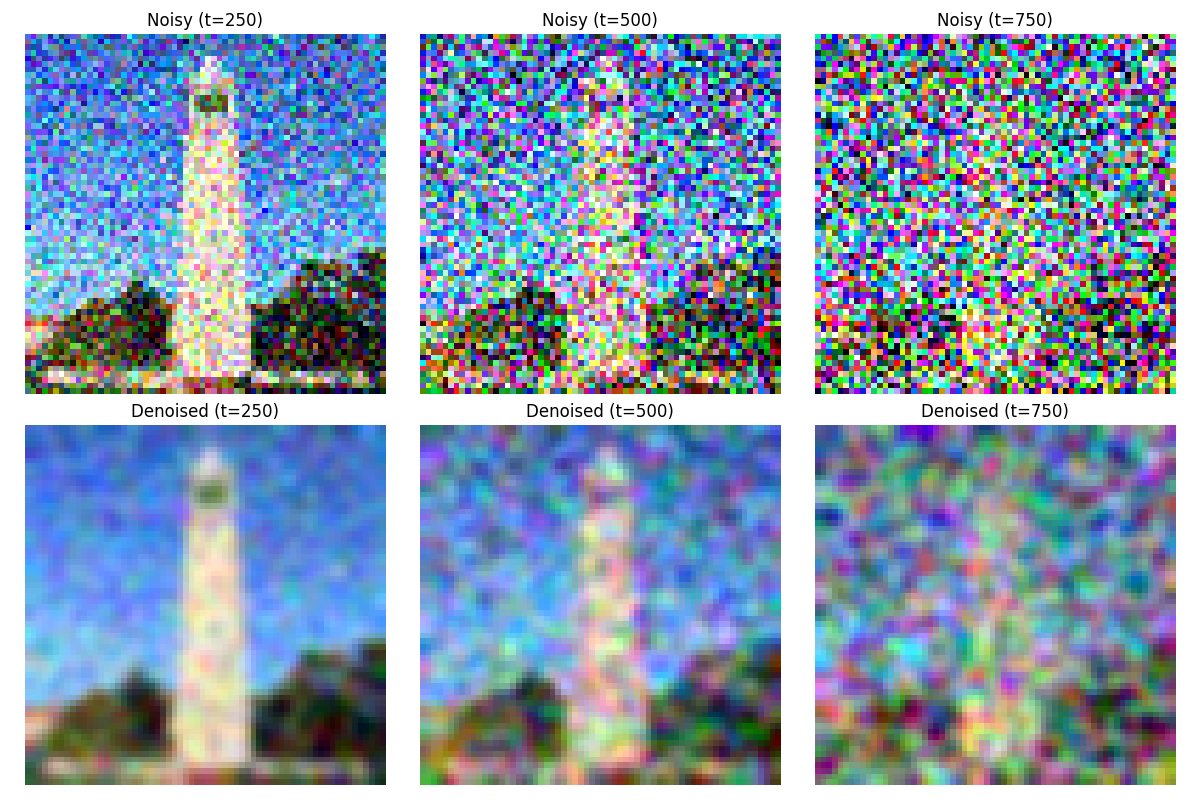
Forward Pass Comparison

Part 1.3: One-Step Denoising

This part implements the one-step denoising by passing the noisy images through a trained denoising model. The denoising model is a simple MLP that takes in the noisy images and outputs the denoised images. We separately denoise the images at time steps 250, 500, 750.

t = 250:

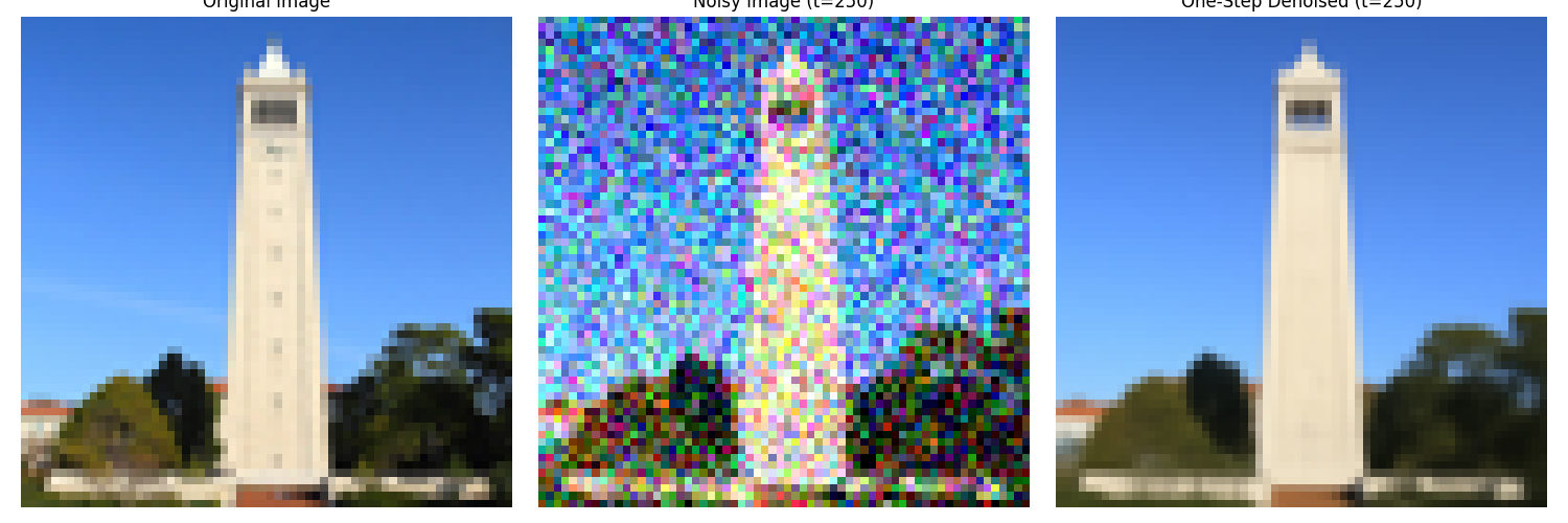
One-Step Denoising at Time Step 250

t = 500:

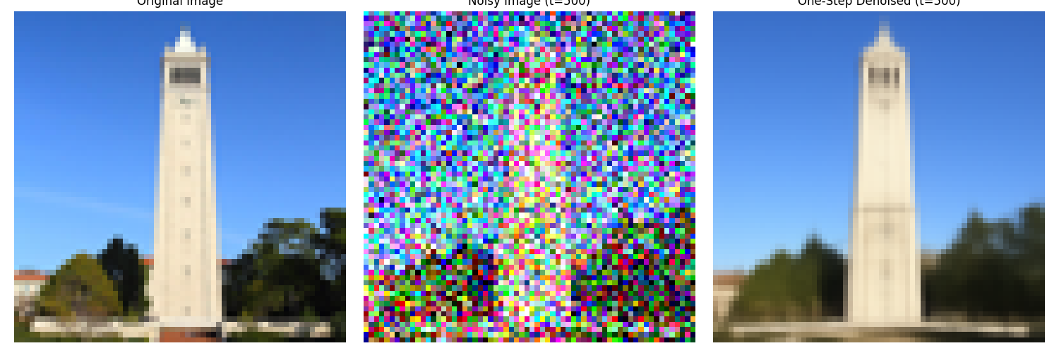
One-Step Denoising at Time Step 500

t = 750:

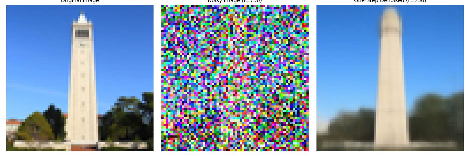
One-Step Denoising at Time Step 750

Part 1.4: Iterative Denoising

While the quality of the one-step denoising is not very good, we can improve it by iterating the denoising process. The iterative denoising process is implemented by passing the noisy images through the denoising model multiple times. We separately denoise the images at time steps 250, 500, 750. The formula for iterative denoising is given by:

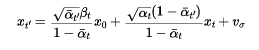
Iterative Denoising

We show the noisy Campanile image during the iterative denoising process.

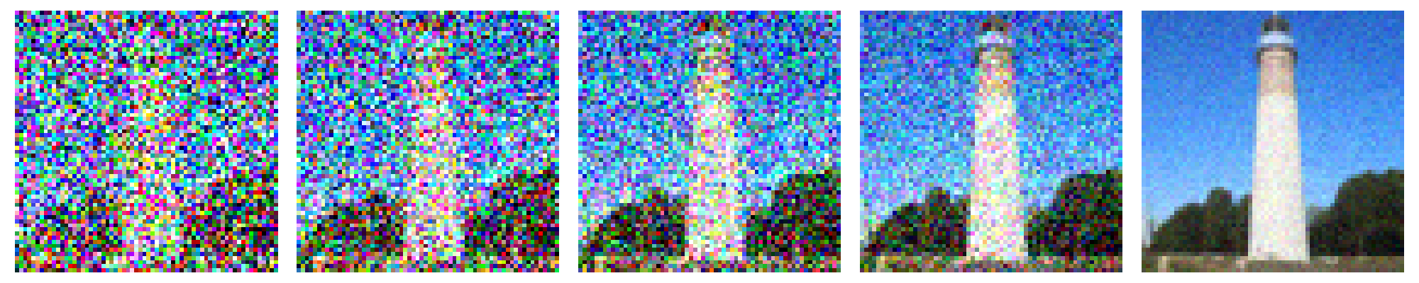
Iterative Denoising Process

Here is a comparison between the classical denoising, the one-step denoising and the iterative denoising.

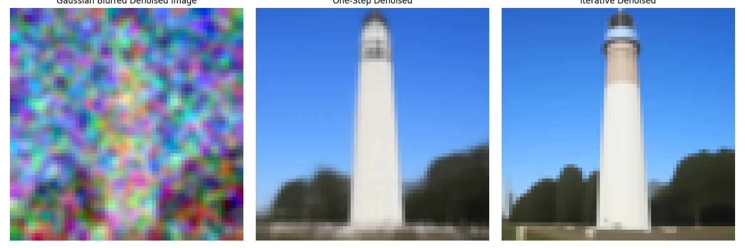
Comparison between the Classical Denoising, the One-Step Denoising and the Iterative Denoising

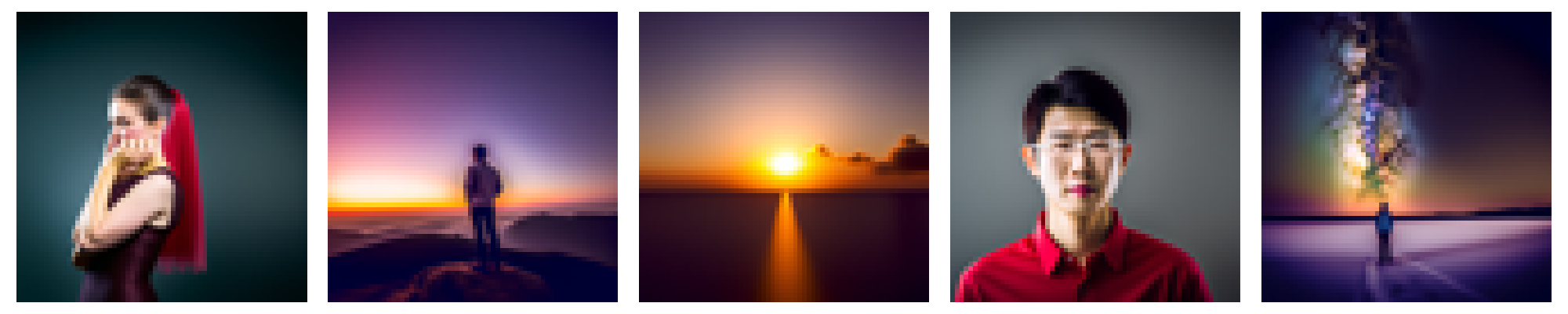
Part 1.5: Diffusion Model Sampling

Here are five sampled images from the diffusion model with the prompt "a high quality photo."

Diffusion Model Sampling

Part 1.6: Classifier-Free Guidance

This part implements the classifier-free guidance by estimating the noise with the following formula:

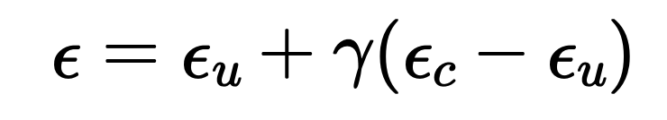
Classifier-Free Guidance

Classifier-Free Guidance

Part 1.7.1: Image-to-Image Translation

The following images are results from the image-to-image translation. It includes the Campanile image, a web imgae, and two hand-drawn images.

Campanile Image, i_start = 1

Campanile Image, i_start = 3

Campanile Image, i_start = 5

Campanile Image, i_start = 7

Campanile Image, i_start = 10

Campanile Image, i_start = 20

Campanile Image, original

Tom and Jerry, i_start = 1

Tom and Jerry, i_start = 3

Tom and Jerry, i_start = 5

Tom and Jerry, i_start = 7

Tom and Jerry, i_start = 10

Tom and Jerry, i_start = 20

Tom and Jerry, original

Drawn Cat, i_start = 1

Drawn Cat, i_start = 3

Drawn Cat, i_start = 5

Drawn Cat, i_start = 7

Drawn Cat, i_start = 10

Drawn Cat, i_start = 20

Drawn Cat, original

Drawn Doraemon, i_start = 1

Drawn Doraemon, i_start = 3

Drawn Doraemon, i_start = 5

Drawn Doraemon, i_start = 7

Drawn Doraemon, i_start = 10

Drawn Doraemon, i_start = 20

Drawn Doraemon, original

Part 1.7.2: Inpainting

This section implements the inpainting technique. in every denoising step, we denoise the whole image. However, only the area with a mask value of 1 is kept. Other areas are reobtained in the next step from redoing the forward pass on the original image. This achieves the effect of only diffusing the masked area with the context unchanged. The following images are examples of the impainted images.

Campanile Image, Original

Campanile Image, Mask

Campanile Image, To Replace

Campanile Image, Inpainted

Dog Image, Original

Dog Image, Mask

Dog Image, To Replace

Dog Image, Inpainted

Charger Image, Original

Charger Image, Mask

Charger Image, To Replace

Charger Image, Inpainted

Part 1.7.3: Text-Conditional Image-to-image Translation

This section is very similar to the image-to-image translation task. The only difference is that in this task, we use a custom textual prompt instead of a general prompt. The following images are examples of the text-conditional image-to-image translation.

Campanile, i_start = 1

Campanile, i_start = 3

Campanile, i_start = 5

Campanile, i_start = 7

Campanile, i_start = 10

Campanile, i_start = 20

Campanile, original

Car, i_start = 1

Car, i_start = 3

Car, i_start = 5

Car, i_start = 7

Car, i_start = 10

Car, i_start = 20

Car, original

Kiwi, i_start = 1

Kiwi, i_start = 3

Kiwi, i_start = 5

Kiwi, i_start = 7

Kiwi, i_start = 10

Kiwi, i_start = 20

Kiwi, original

Part 1.8: Visual Anagrams

This section implements the visual anagrams. In every denoising step, we predict the normal noise and we also predict the noise flipped based on the flipped prompt. We then simply flip the flipped noise back and add them together to get our final perdicted noise. The process is given by the following formula:

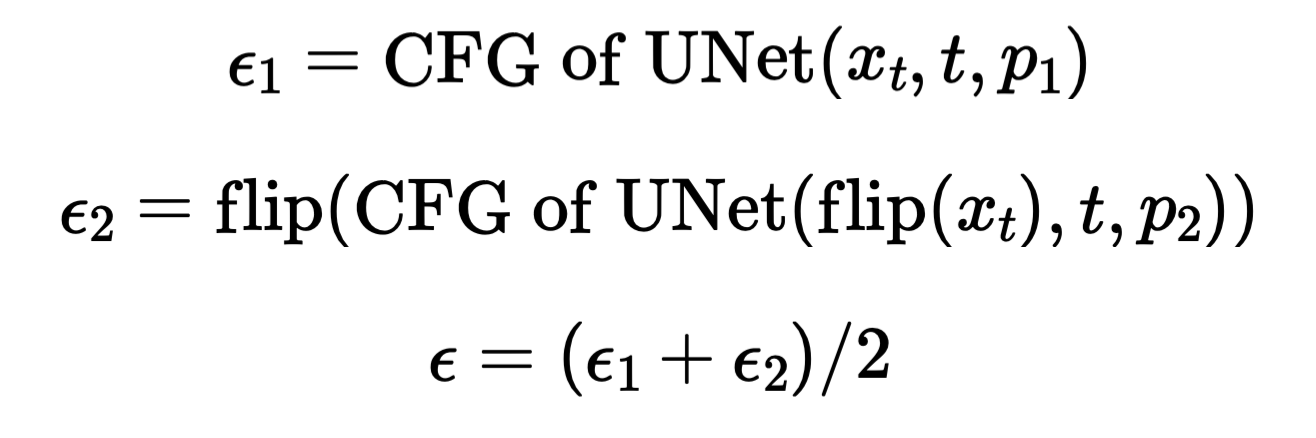
Classifier-Free Guidance

Flip Illusion, Campfire + Skull

Flip Illusion, Campfire + Skull

Flip Illusion, Old Man + Campfire

Flip Illusion, Old Man + Campfire

Flip Illusion, Old Man + Village

Flip Illusion, Old Man + Village

Part 1.9: Hybrid Images

This section implements hybrid images. This is done by predicting noises both in the low frequency and the high frequency domains. We then add them together to get our final noise. The process is given by the following formula:

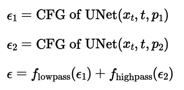
Classifier-Free Guidance

Hybrid Images, Campfire + Skull

Hybrid Images, Rocket Ship + Pencil

Hybrid Images, Skull + Waterfalls

Part B.1.1 and Part B.1.2.0: Implement the UNet and Visualizing the Noisy Images

We add Gaussian noise to the image based on x' = x + l * z, where l is the noise level, z is sampled from a gaussian, x is the original image, and x' is the noisy resulting image. The following images are examples of the noisy images with different noise levels.

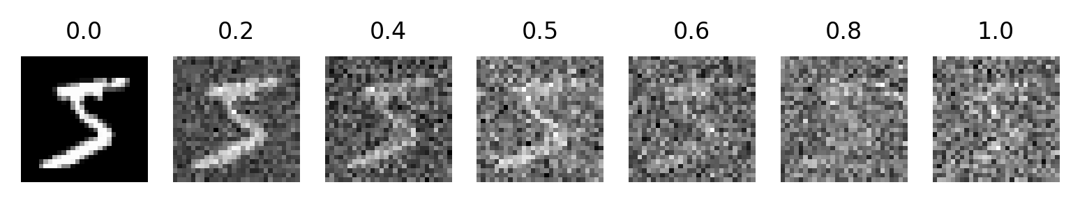
Visualization of the Noisy Images

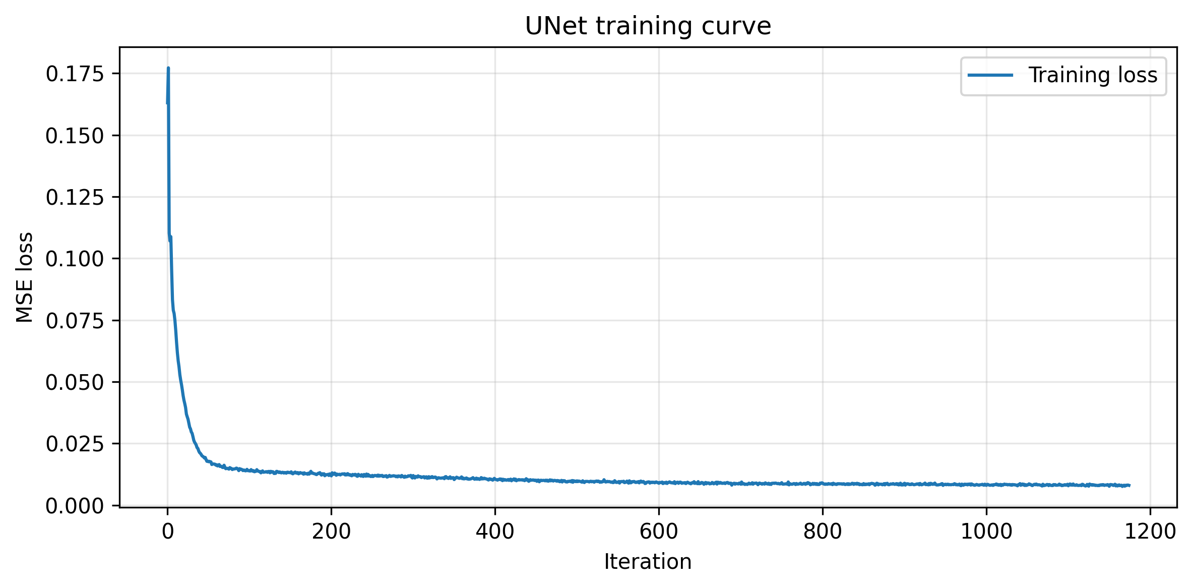
Part B.1.2.1: Training

The UNet is implemented exactly as it shows on the project webpage, with indicidual blocks implemented with PyTorch classes. The UNet is trained on the MNIST dataset with a noise level of 0.5. Here is the training loss curve and the visualization of denoised images after the first and the final epoch.

Trining Loss Curve

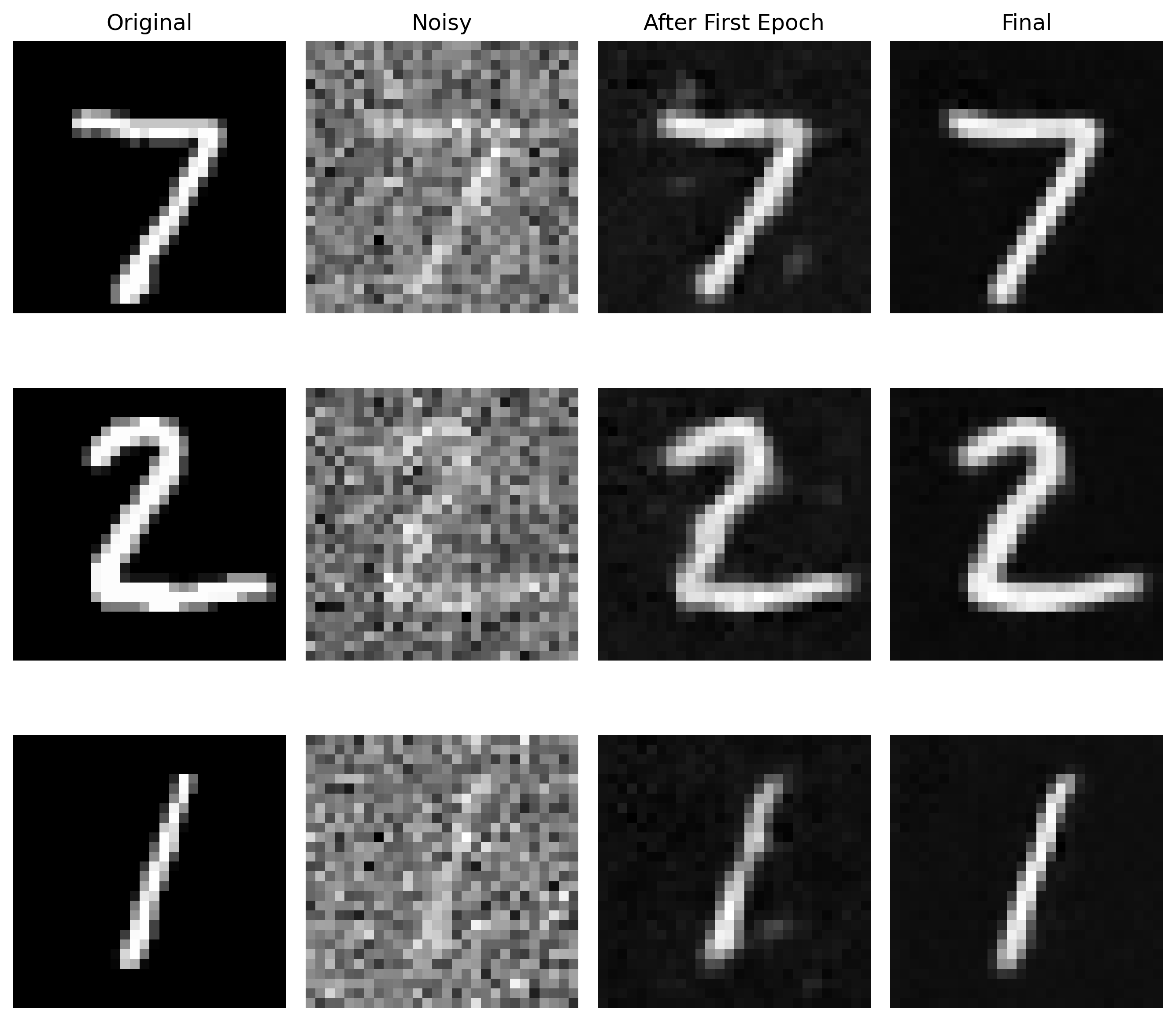
Comparison between the denoised image after the first and the final epoch

Part B.1.2.2: Out-of-Distribution Testing

This section tests the trained UNet's performance on out-of-distribution data, ie. images with different noise levels. With a larger noise level, the denoising performance seems to drop, which makes sense since the model is not trained on such levels.

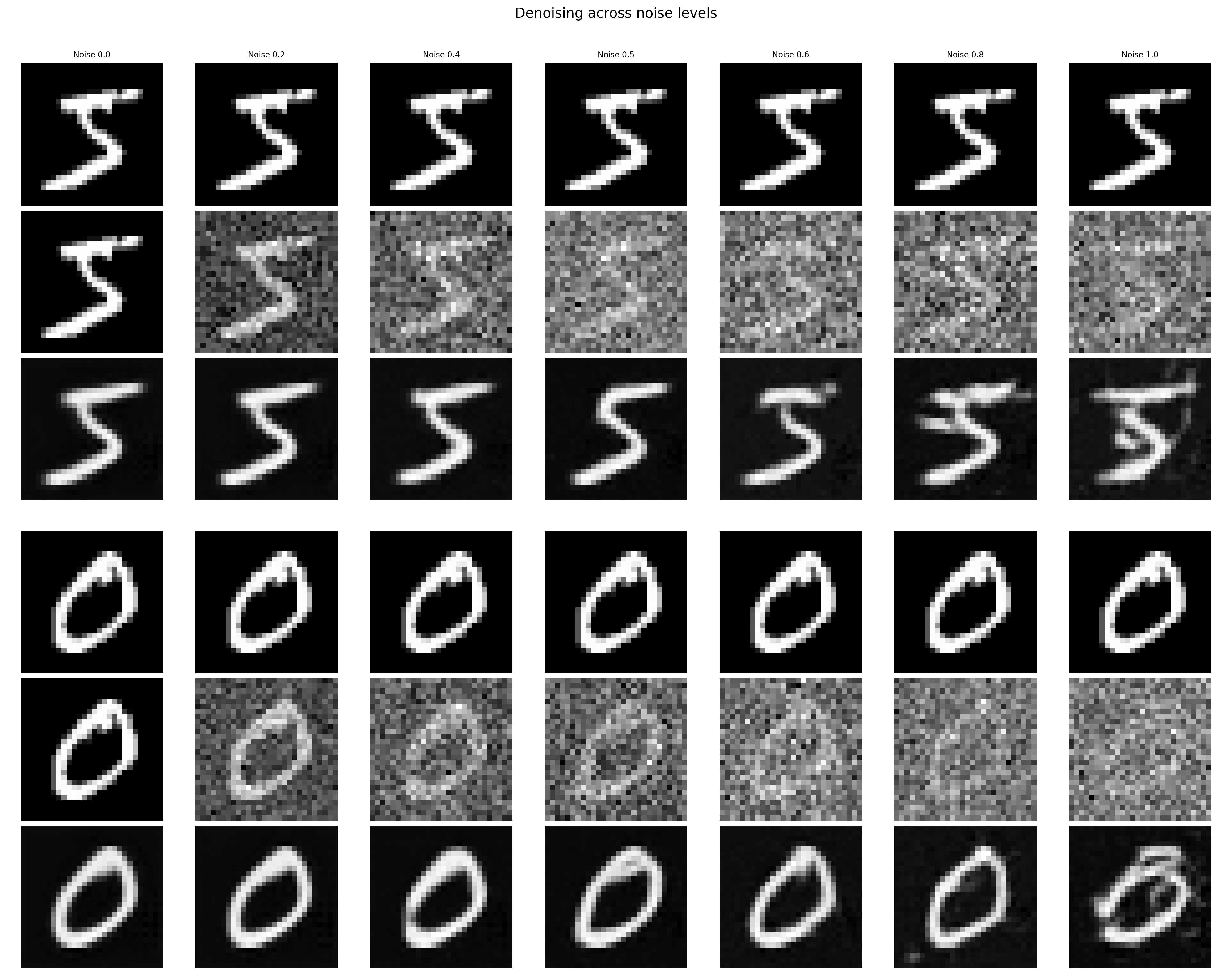
Performance of the denoiser on OOD noise levels

Part B.1.2.3: Denoising Pure Noise

This section trains a UNet to denoise a pure noise. Since the training is not conditioned on the classes, we expect the model to output images that don't look like actual numbers.

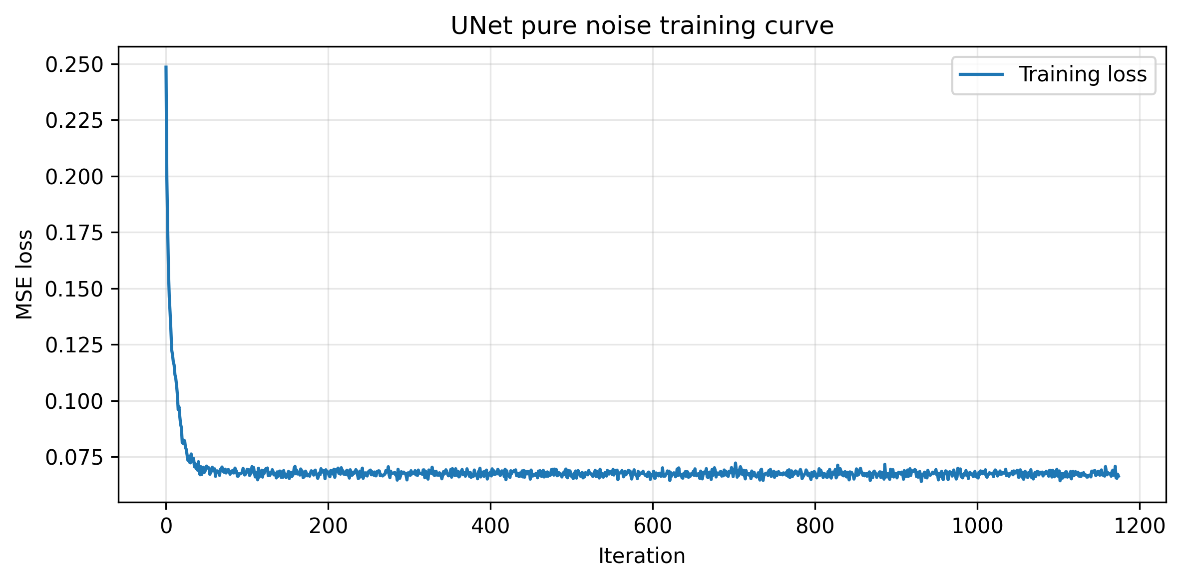
Training Loss Curve for the UNet Trained for Denoising Pure Noises

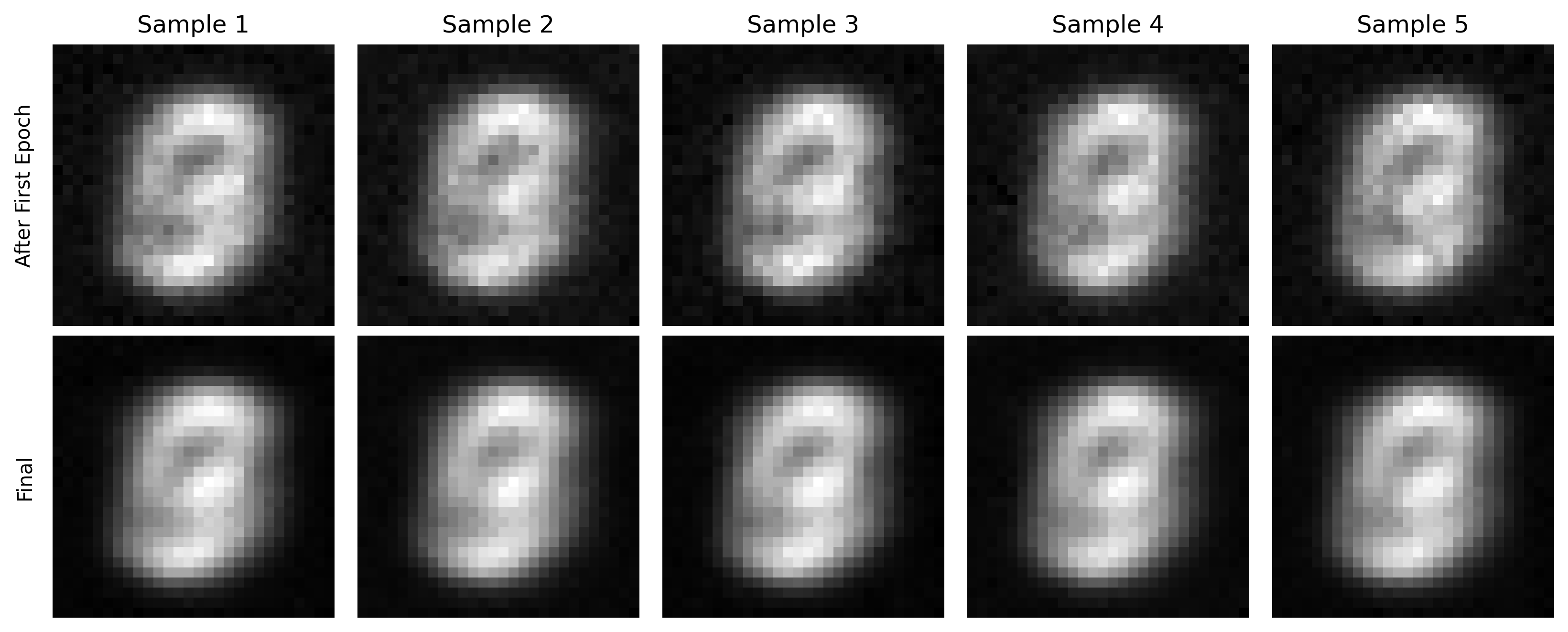
Sampled Results on Pure Noise for the Model after the First and the Final epoch

Notice that the outputted images have features of different numbers in the training dataset. This is because the training is not conditioned on classes; therefore, pure noise can be denoised to any number during the training process.

Part B.2: Training a Flow Matching Model

The one-step denoiser doesn't work well. Therefore, we want to train a denoiser that iteratively denoise the pure noises. We choose to implement the flow matching model in the following sections. We will start with time and class conditioned UNet implementations.

Part B.2.1 and Part B.2.2: Adding Time Conditioning to UNet and Training the UNet

We implement the fully connected block and pass the conditioned time variable before the concatenations. This allows the model to learn which time step is this noisy image on. The training loss curve is presented below.

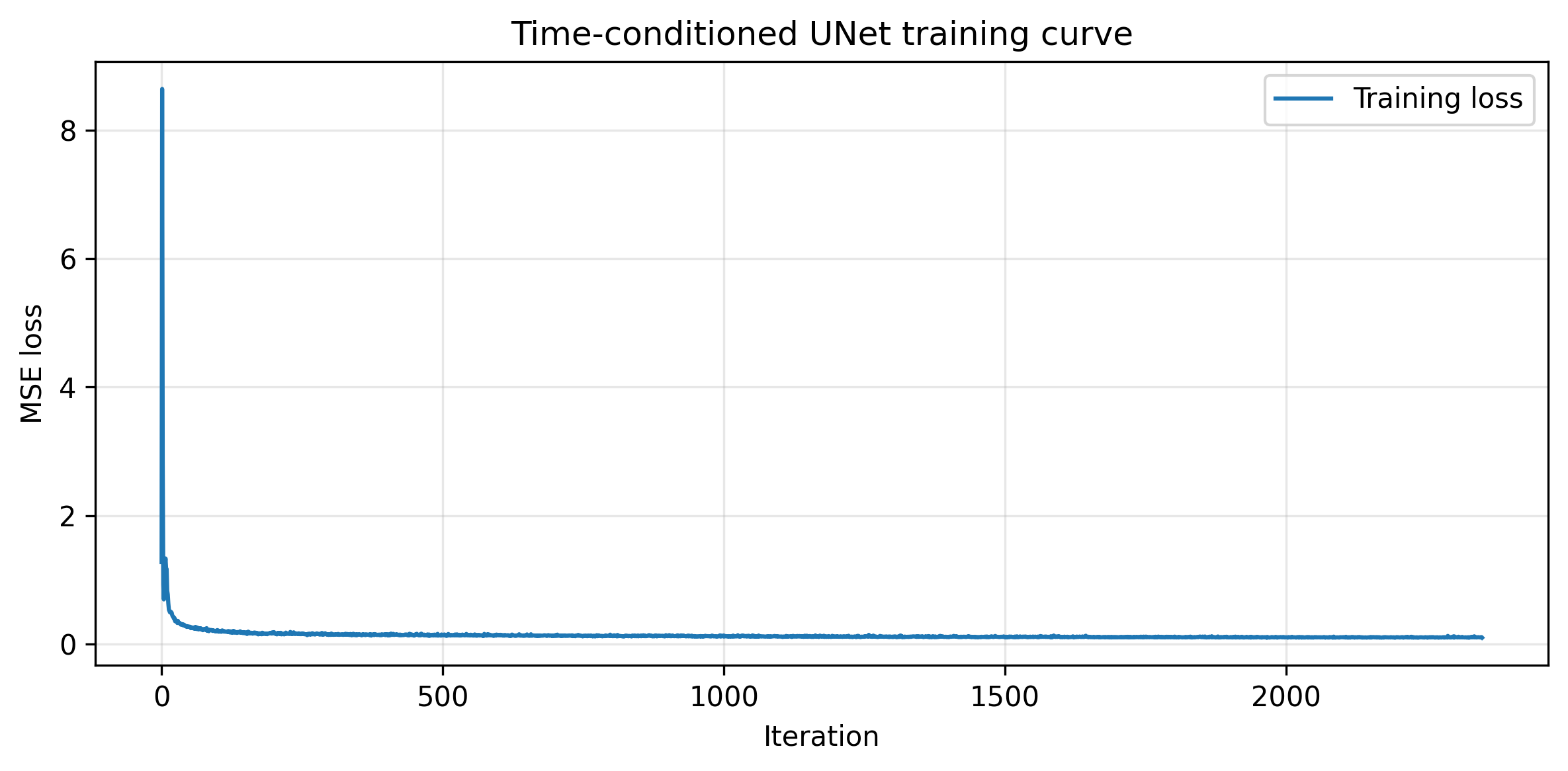
Training Loss Curve for the Time-Conditioned UNet

Part B.2.3: Sampling from the UNet

The following images demonstrate the denoising effects from the trained model after the first, fifth, and the final epoch.

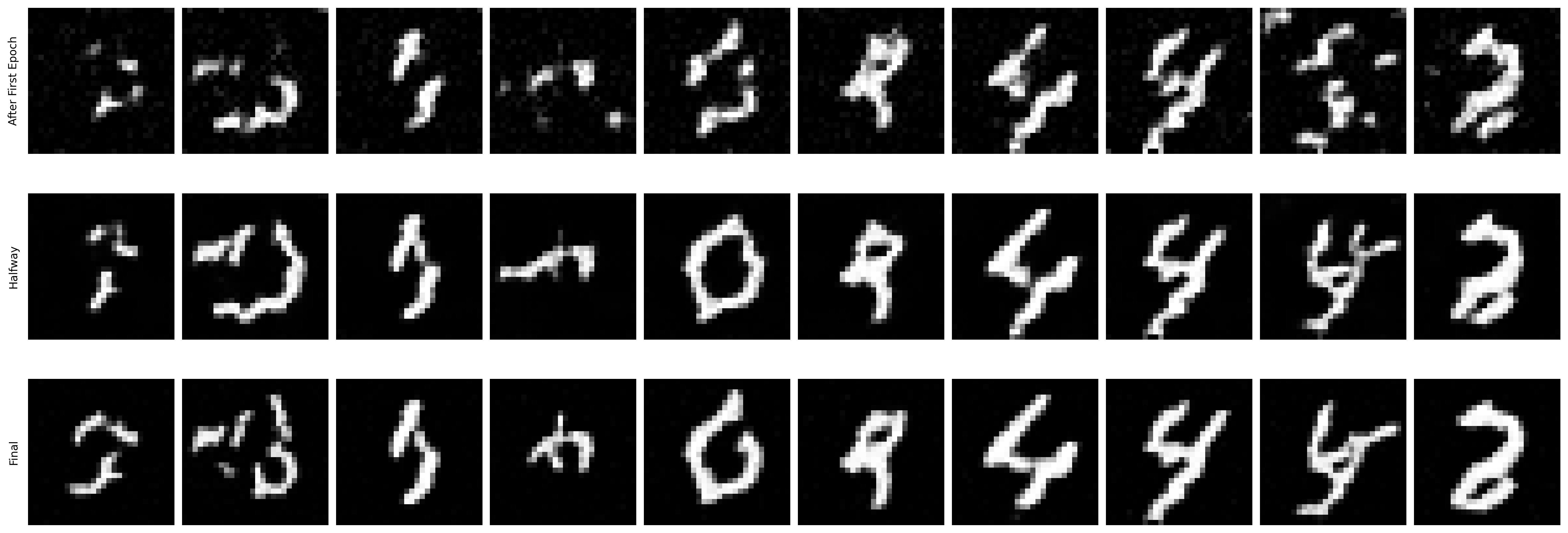
Sampled Results from the Time-Conditioned UNet

Part B.2.4 and Part B.2.5: Adding Class-Conditioning to UNet and Training the UNet

To better generate number images, we can further condition the UNet on the classes. The condition is also added with a fully connected block. Below is the training loss curve of the class-conditioned UNet.

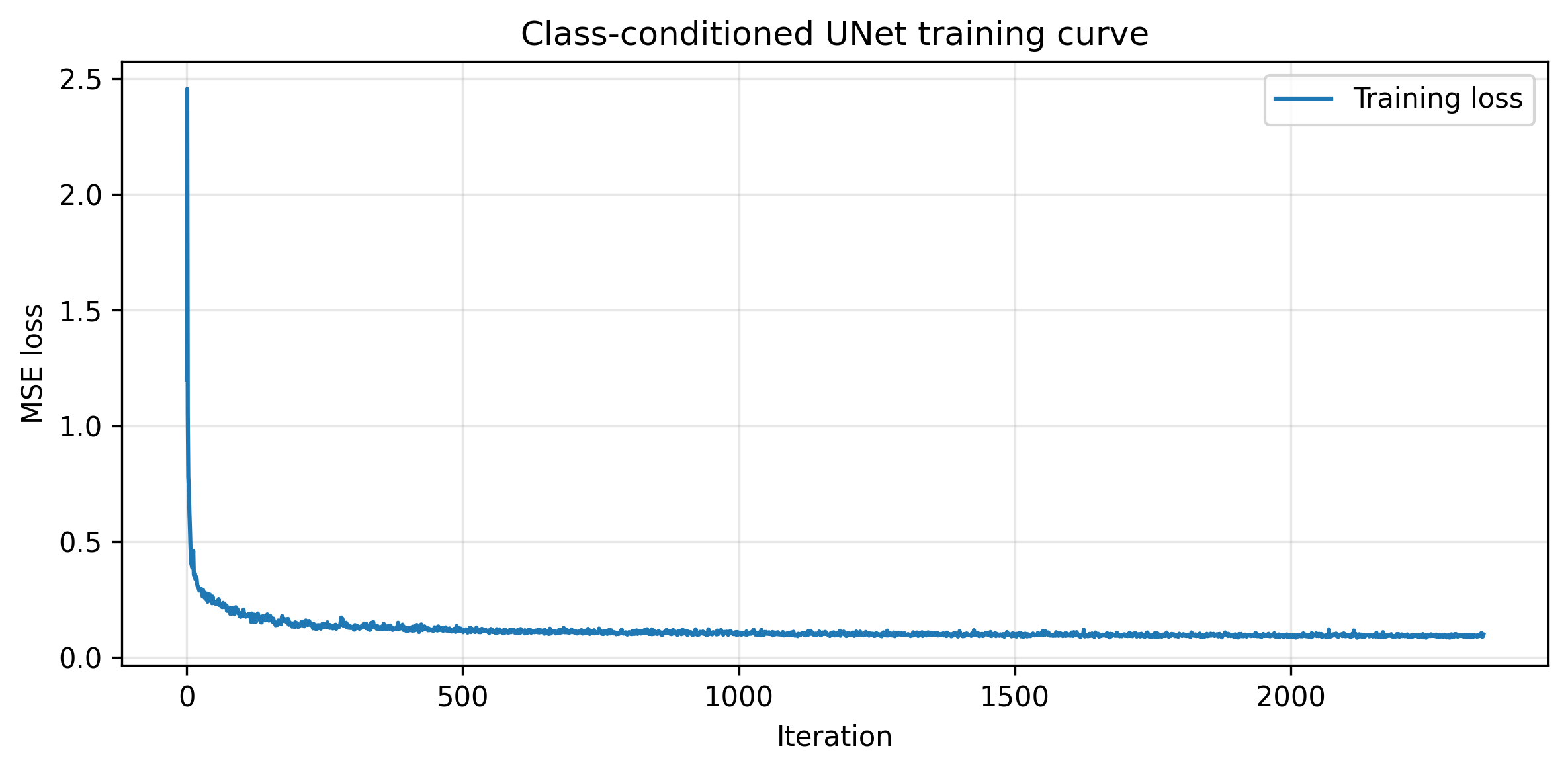
Training Loss Curve for the Time-Conditioned UNet

Part B.2.6: Sampling from the UNet

The following images demonstrate the denoising effects from the trained class-conditioned UNet after the first, fifth, and the final epoch. The more the training steps, the better the sampled results.

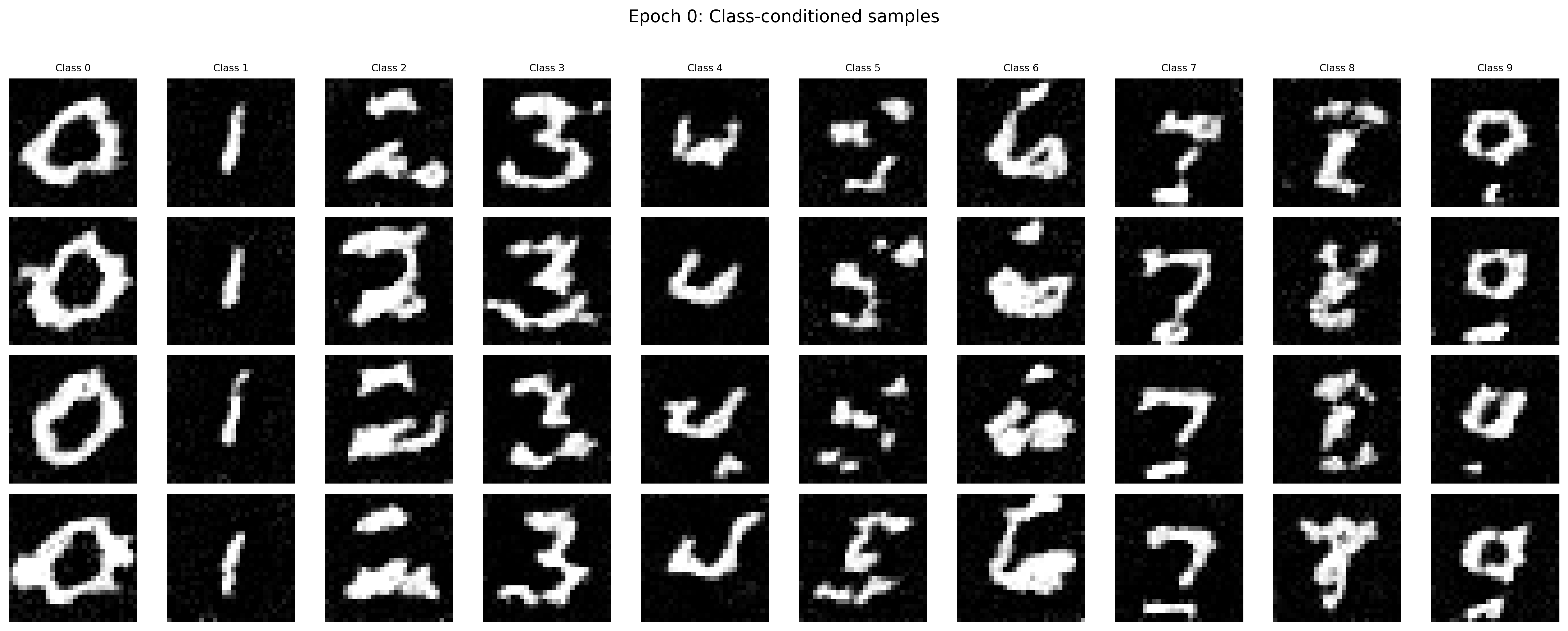
Sampled Results of the Class-Conditioned Unet after the First Epoch

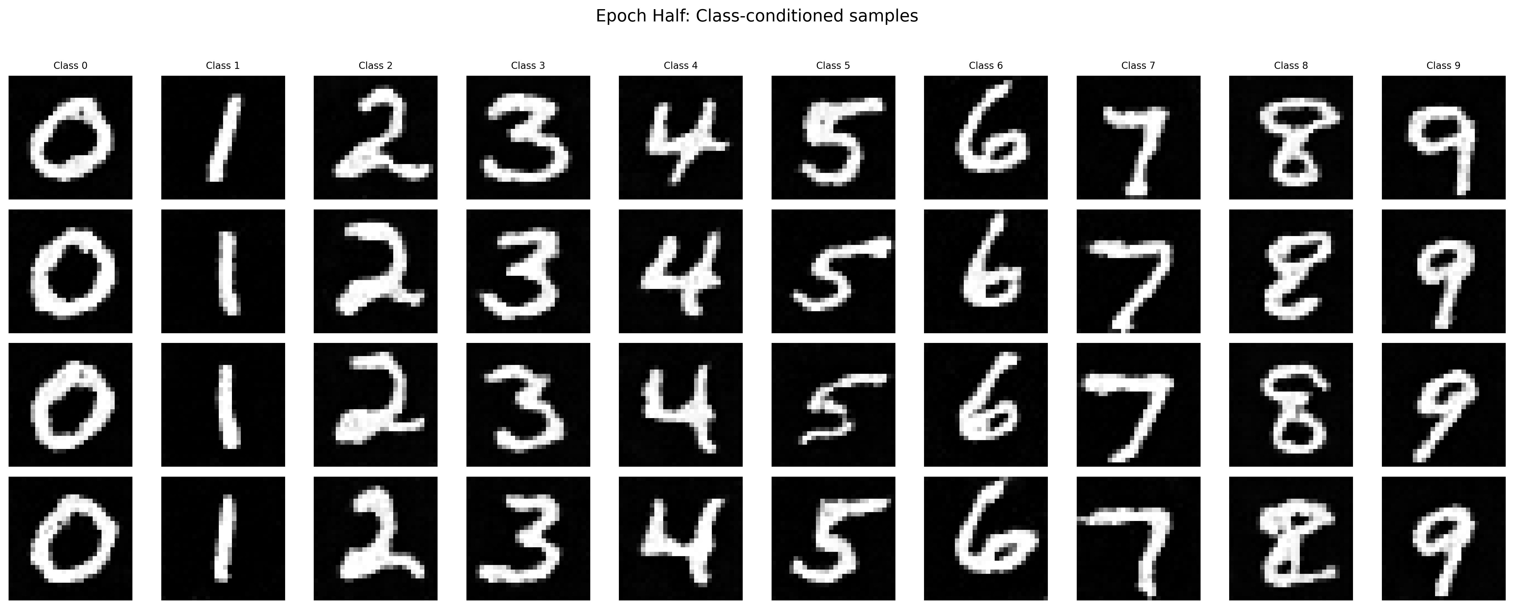
Sampled Results of the Class-Conditioned Unet after the Fifth Epoch

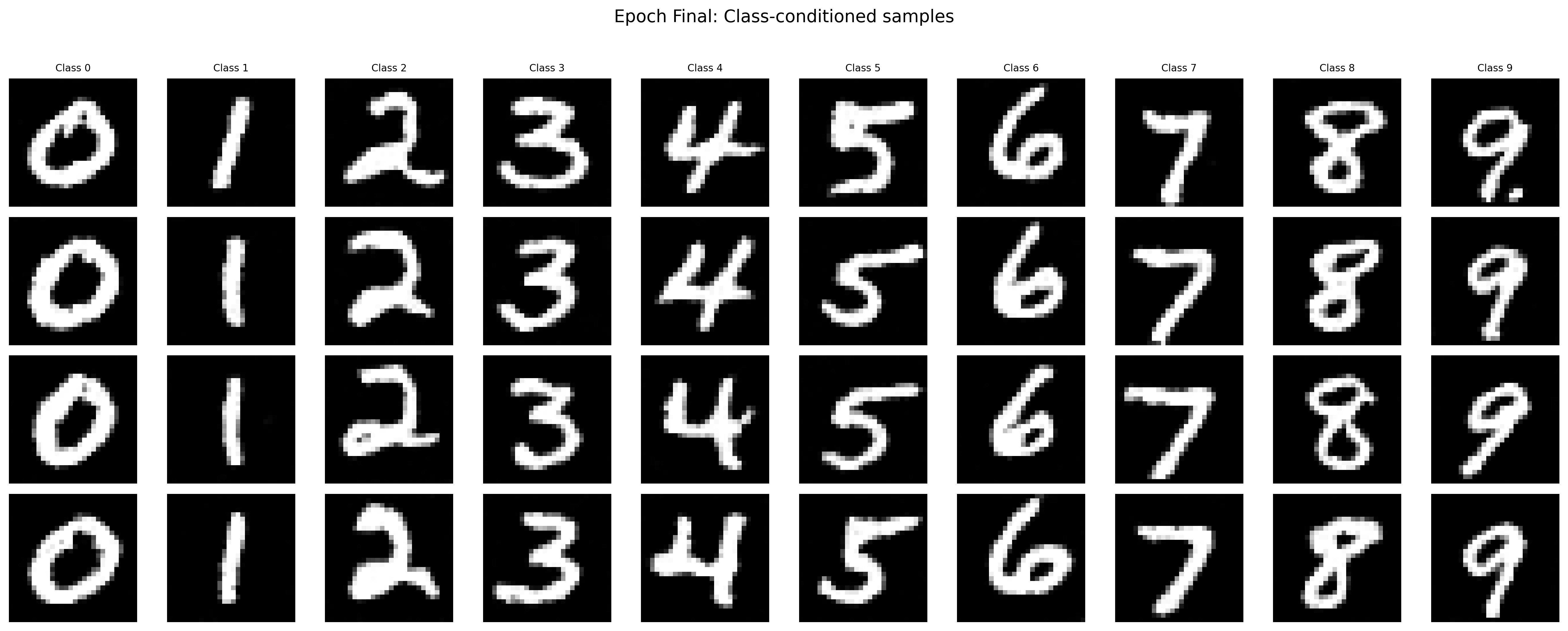
Sampled Results of the Class-Conditioned Unet after the Final Epoch

To keep the training process simple, we can get rid of the scheduler and use a constant learning rate instead (perhaps with a smaller learning rate and more training steps). I choose to train the model with a constant learning rate of 1e-3 for 20 epochs. The following images demonstrate the training and sampled results.

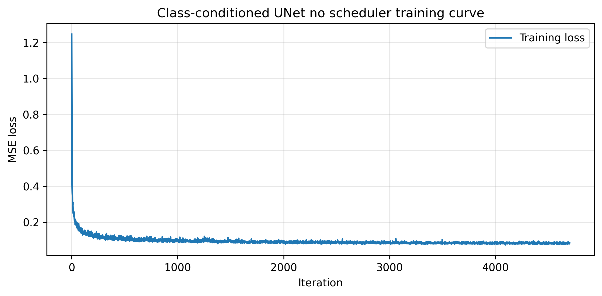
Training Loss Curve for the Class-Conditioned UNet without the Scheduler

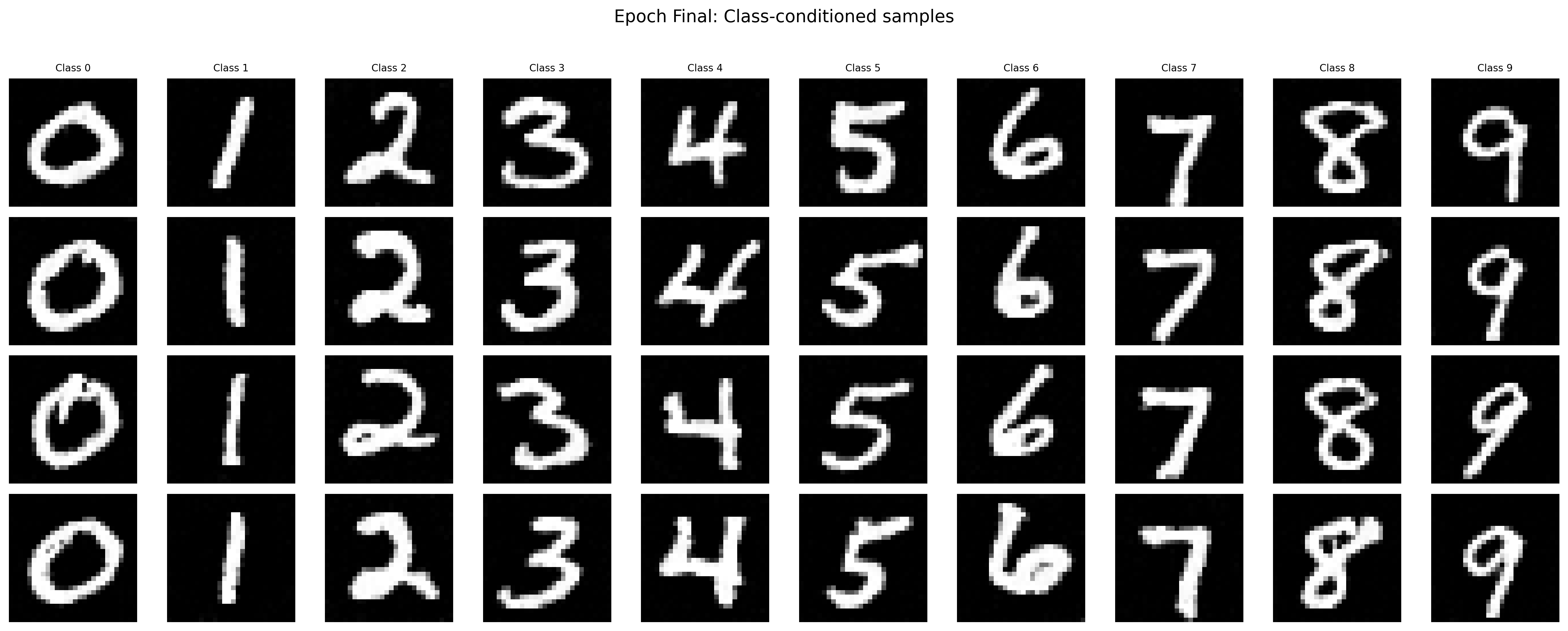
Sampled Results of the Class-Conditioned Unet after the Final Epoch without the Scheduler